Welcome to the spatialLIBD project! It is composed of the HumanPilot
described here as well as:
- a shiny web application that we are hosting at spatial.libd.org/spatialLIBD/ that can handle a limited set of concurrent users,
- a Bioconductor package at bioconductor.org/packages/spatialLIBD (or from here) that lets you analyze the data and run a local version of our web application (with our data or yours),
- and a research article with the scientific knowledge we drew from this dataset. The analysis code for our project is available here that you are looking at right now.
This web application allows you to browse the LIBD human dorsolateral pre-frontal cortex (DLPFC) spatial transcriptomics data generated with the 10x Genomics Visium platform. Through the R/Bioconductor package you can also download the data as well as visualize your own datasets using this web application. Please check the bioRxiv pre-print for more details about this project.
If you tweet about this website, the data or the R package please use
the #spatialLIBD hashtag. You can find previous tweets
that way as shown
here.
Thank you!
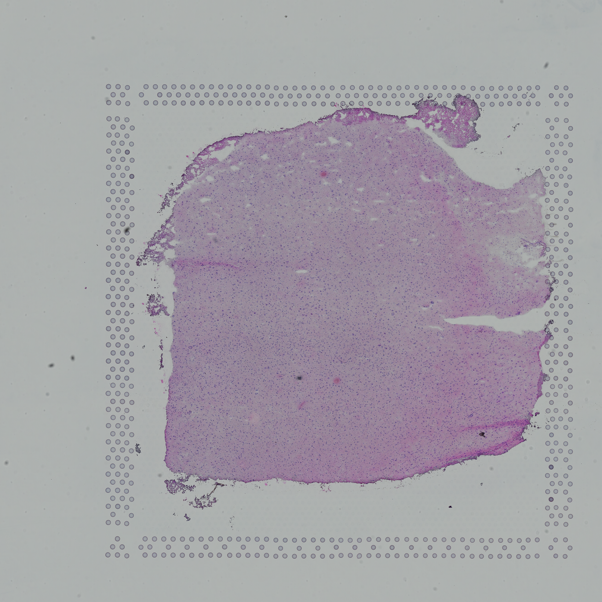
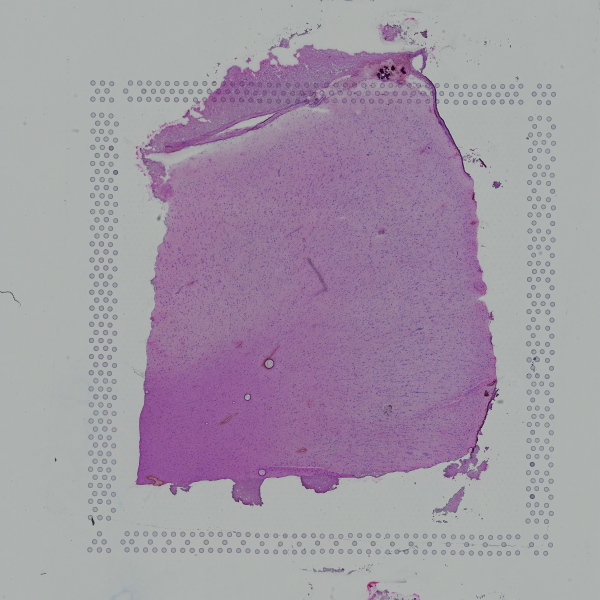
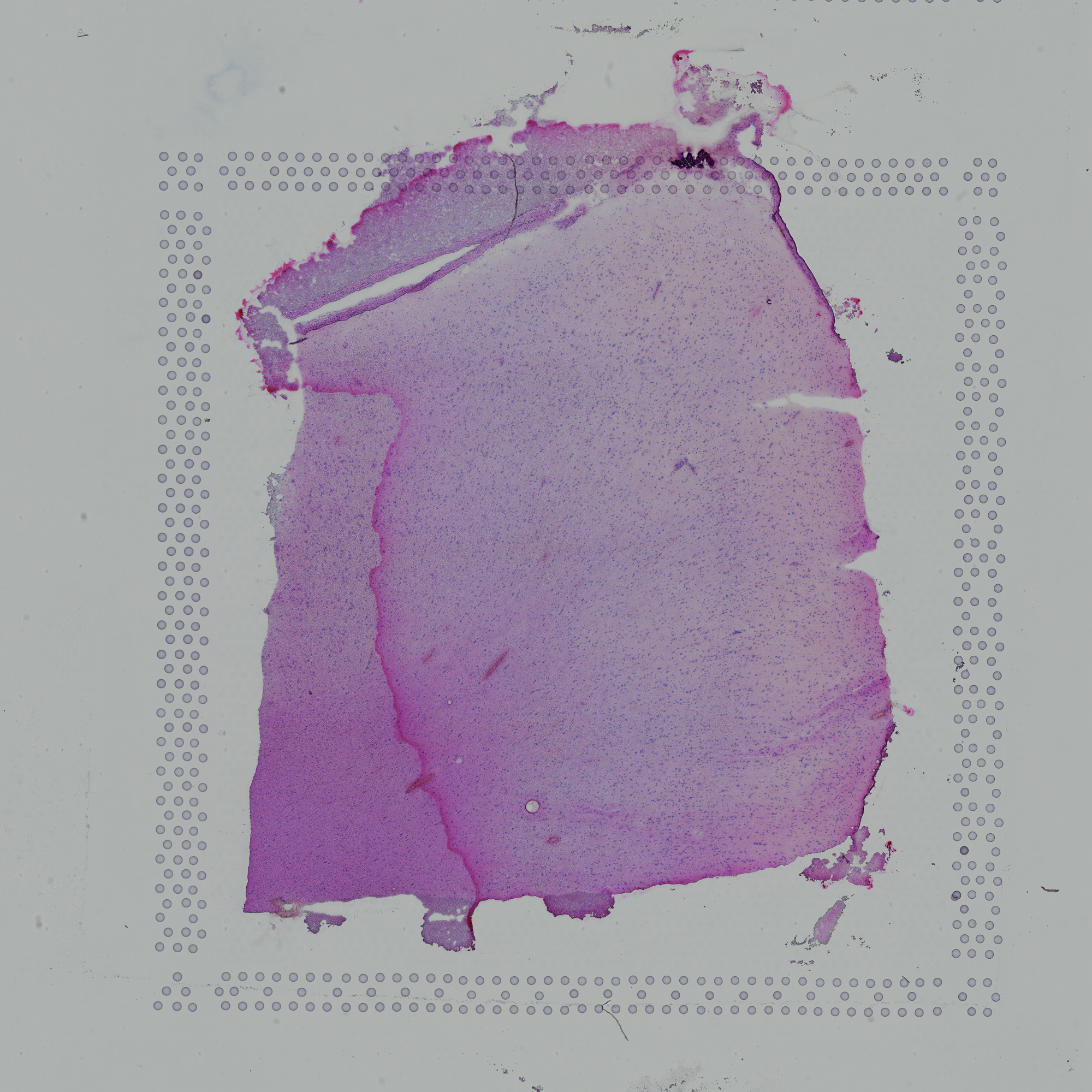
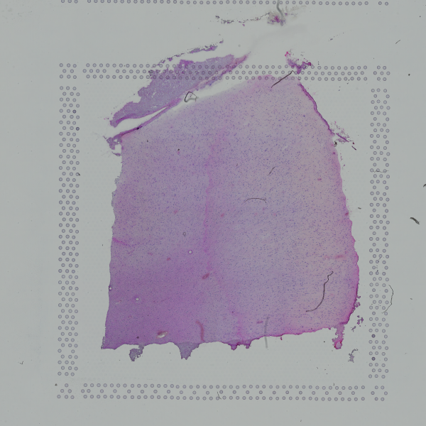
As a quick overview, the data presented here is from portion of the DLPFC that spans six neuronal layers plus white matter (A) for a total of three subjects with two pairs of spatially adjacent replicates (B). Each dissection of DLPFC was designed to span all six layers plus white matter (C). Using this web application you can explore the expression of known genes such as SNAP25 (D, a neuronal gene), MOBP (E, an oligodendrocyte gene), and known layer markers from mouse studies such as PCP4 (F, a known layer 5 marker gene).
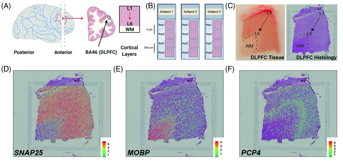
This web application was built such that we could annotate the spots to layers as you can see under the spot-level data tab. Once we annotated each spot to a layer, we compressed the information by a pseudo-bulking approach into layer-level data. We then analyzed the expression through a set of models whose results you can also explore through this web application. Finally, you can upload your own gene sets of interest as well as layer enrichment statistics and compare them with our LIBD Human DLPFC Visium dataset.
If you are interested in running this web application locally, you can
do so thanks to the spatialLIBD R/Bioconductor package that powers
this web application as shown below.
## Run this web application locally
spatialLIBD::run_app()

## You will have more control about the length of the
## session and memory usage.

## You could also use this function to visualize your
## own data given some requirements described
## in detail in the package vignette documentation
## at http://research.libd.org/spatialLIBD/.The spatialLIBD package contains functions for:
- Accessing the spatial transcriptomics data from the LIBD Human Pilot
project (code on
GitHub) generated
with the Visium platform from 10x Genomics. The data is retrieved
from Bioconductor’s
ExperimentHub. - Visualizing the spot-level spatial gene expression data and clusters.
- Inspecting the data interactively either on your computer or through spatial.libd.org/spatialLIBD/.
For more details, please check the documentation website or the Bioconductor package landing page here.
Get the latest stable R release from
CRAN. Then install spatialLIBD using
from Bioconductor the following code:
if (!requireNamespace("BiocManager", quietly = TRUE))
    install.packages("BiocManager")

BiocManager::install("spatialLIBD")Through the spatialLIBD package you can access the processed data in
it’s final R format. However, we also provide a table of links so you
can download the raw data we received from 10x Genomics.
Using spatialLIBD you can access the Human DLPFC spatial
transcriptomics data from the 10x Genomics Visium platform. For example,
this is the code you can use to access the layer-level data. For more
details, check the help file for fetch_data().
## Load the package
library("spatialLIBD")
## Download the spot-level data
spe <- fetch_data(type = "spe")
## This is a SpatialExperiment object
spe
#> class: SpatialExperiment
#> dim: 33538 47681
#> metadata(0):
#> assays(2): counts logcounts
#> rownames(33538): ENSG00000243485 ENSG00000237613 ... ENSG00000277475
#> ENSG00000268674
#> rowData names(9): source type ... gene_search is_top_hvg
#> colnames(47681): AAACAACGAATAGTTC-1 AAACAAGTATCTCCCA-1 ...
#> TTGTTTCCATACAACT-1 TTGTTTGTGTAAATTC-1
#> colData names(66): sample_id Cluster ... spatialLIBD ManualAnnotation
#> reducedDimNames(6): PCA TSNE_perplexity50 ... TSNE_perplexity80
#> UMAP_neighbors15
#> mainExpName: NULL
#> altExpNames(0):
#> spatialData names(3) : in_tissue array_row array_col
#> spatialCoords names(2) : pxl_col_in_fullres pxl_row_in_fullres
#> imgData names(4): sample_id image_id data scaleFactor
## Note the memory size
lobstr::obj_size(spe)
#> 2.04 GB
## Remake the logo image with histology information
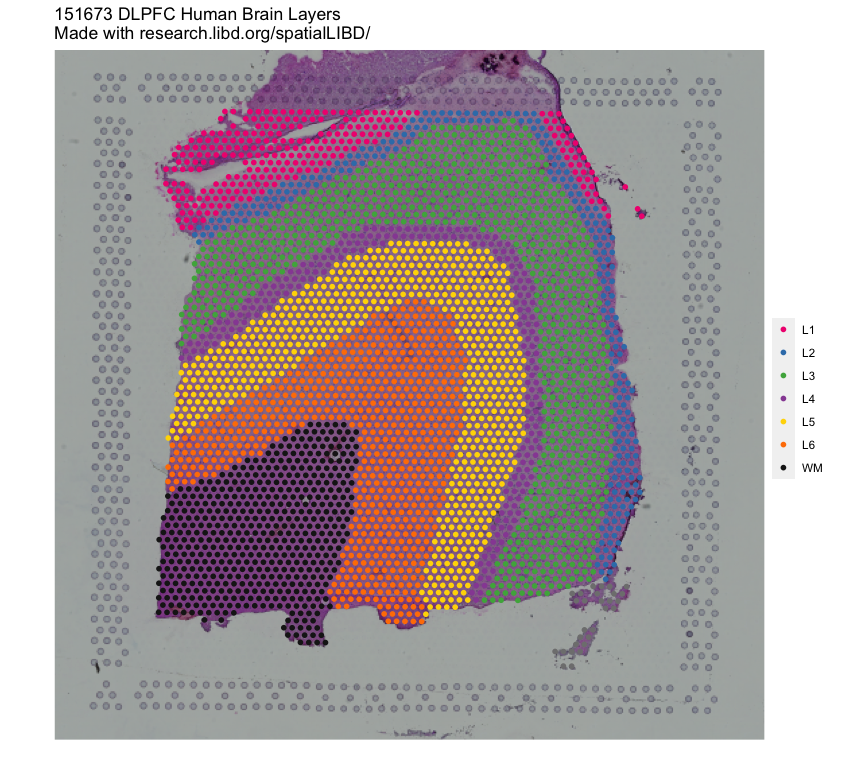
vis_clus(
spe = spe,
clustervar = "spatialLIBD",
sampleid = "151673",
colors = libd_layer_colors,
... = " DLPFC Human Brain Layers\nMade with github.com/LieberInstitute/spatialLIBD"
)
You can access all the raw data through
Globus (jhpce#HumanPilot10x).
Furthermore, below you can find the links to the raw data we received
from 10x Genomics.
| SampleID | h5_filtered | h5_raw | image_full | image_hi | image_lo | loupe | HTML_report |
|---|---|---|---|---|---|---|---|
| 151507 | AWS | AWS | AWS | AWS | AWS | AWS | GitHub |
| 151508 | AWS | AWS | AWS | AWS | AWS | AWS | GitHub |
| 151509 | AWS | AWS | AWS | AWS | AWS | AWS | GitHub |
| 151510 | AWS | AWS | AWS | AWS | AWS | AWS | GitHub |
| 151669 | AWS | AWS | AWS | AWS | AWS | AWS | GitHub |
| 151670 | AWS | AWS | AWS | AWS | AWS | AWS | GitHub |
| 151671 | AWS | AWS | AWS | AWS | AWS | AWS | GitHub |
| 151672 | AWS | AWS | AWS | AWS | AWS | AWS | GitHub |
| 151673 | AWS | AWS | AWS | AWS | AWS | AWS | GitHub |
| 151674 | AWS | AWS | AWS | AWS | AWS | AWS | GitHub |
| 151675 | AWS | AWS | AWS | AWS | AWS | AWS | GitHub |
| 151676 | AWS | AWS | AWS | AWS | AWS | AWS | GitHub |
Below is the citation output from using citation('spatialLIBD') in R.
Please run this yourself to check for any updates on how to cite
spatialLIBD.
citation('spatialLIBD')
#>
#> To cite package 'spatialLIBD' in publications use:
#>
#>   Pardo B, Spangler A, Weber LM, Hicks SC, Jaffe AE, Martinowich K,
#>   Maynard KR, Collado-Torres L (2022). "spatialLIBD: an R/Bioconductor
#>   package to visualize spatially-resolved transcriptomics data." _BMC
#>   Genomics_. doi:10.1186/s12864-022-08601-w
#>   <https://doi.org/10.1186/s12864-022-08601-w>,
#>   <https://doi.org/10.1186/s12864-022-08601-w>.
#>
#>   Maynard KR, Collado-Torres L, Weber LM, Uytingco C, Barry BK,
#>   Williams SR, II JLC, Tran MN, Besich Z, Tippani M, Chew J, Yin Y,
#>   Kleinman JE, Hyde TM, Rao N, Hicks SC, Martinowich K, Jaffe AE
#>   (2021). "Transcriptome-scale spatial gene expression in the human
#>   dorsolateral prefrontal cortex." _Nature Neuroscience_.
#>   doi:10.1038/s41593-020-00787-0
#>   <https://doi.org/10.1038/s41593-020-00787-0>,
#>   <https://www.nature.com/articles/s41593-020-00787-0>.
#>
#> To see these entries in BibTeX format, use 'print(<citation>,
#> bibtex=TRUE)', 'toBibtex(.)', or set
#> 'options(citation.bibtex.max=999)'.As described in the spatialLIBD vignette, you can see the scripts in
this repository for re-shaping your data to look like ours. That is.
reorganize_folder.Ravailable here re-organizes the raw data we were sent by 10x Genomics.Layer_Notebook.Ravailable here reads in the Visium data and builds a list ofRangeSummarizedExperiment()objects from SummarizedExperiment, one per sample (image) that is eventually saved asHuman_DLPFC_Visium_processedData_rseList.rda.convert_sce.Ravailable here reads inHuman_DLPFC_Visium_processedData_rseList.rdaand builds an initialsceobject with image data undermetadata(sce)$imagewhich is a single data.frame. Subsetting doesn’t automatically subset the image, so you have to do it yourself when plotting as is done bysce_image_clus_p()andsce_image_gene_p(). Having the data from all images in a single object allows you to use the spot-level data from all images to compute clusters and do other similar analyses to the ones you would do with sc/snRNA-seq data. The script creates theHuman_DLPFC_Visium_processedData_sce.Rdatafile.sce_scran.Ravailable here then uses scran to read inHuman_DLPFC_Visium_processedData_sce.Rdata, compute the highly variable genes (stored in our finalsceobject atrowData(sce)$is_top_hvg), perform dimensionality reduction (PCA, TSNE, UMAP) and identify clusters using the data from all images. The resulting data is then stored asHuman_DLPFC_Visium_processedData_sce_scran.Rdataand is the main object used throughout our analysis code (Maynard, Collado-Torres, Weber, Uytingco, et al., 2021).make-data_spatialLIBD.Ravailable in the source version ofspatialLIBDand online here is the script that reads inHuman_DLPFC_Visium_processedData_sce_scran.Rdataas well as some other outputs from our analysis and combines them into the finalsceandsce_layerobjects provided by spatialLIBD (Pardo, Spangler, Weber, Hicks, et al., 2022). This script simplifies some operations in order to simplify the code behind the shiny application provided by spatialLIBD.
10X directory
Contains some of the raw files provided by 10X. Given their size, we only included the small ones here. ## Analysis directory
The README.md was the one we initially prepared for our collaborators
at an early stage of the project. That README file described some of our
initial explorations using packages such as
scran,
zinbwave and other
approaches such as using k-means with X/Y spatial information. These
analyses were not used for our manuscript beyond creating the sce
object we previously described.
The 10x Genomics file structure is replicated inside
Histology where we saved the image segmentation
analysis output to estimate the number of cells per spot. This involved
running some histology image segmentation
software
and the counting code that requires our file
structure (sgeID input).
The main layer-level analysis code is located at
Layer_Guesses, for example
layer_specificity.R is the
R script for pseudo-bulking the spot-level data to create the
layer-level data. The spatialLIBD layer annotation files are saved in
the First_Round and
Second_Round directories which
you can upload to the shiny web application.
We also include directories with code for processing external datasets such as he_layers, allen_data, hafner_vglut.
We would like to highlight that a lot of the plotting code and functionality from these scripts has been implemented in spatialLIBD which would make a lot of our analysis simpler. Finally, for reproducibility purposes we included the R session information in many of our R scripts. Although in general we used R 3.6.1 and 3.6.2 with Bioconductor release 3.10.
outputs directory
Contains outputs from the different unsupervised, semi-supervised, known gene marker based and other clustering results. The analysis code that generates these CSV files is located inside R Markdown files at the Analysis directory such as SpatialDE_clustering.Rmd.
[1] K. R. Maynard, L. Collado-Torres, L. M. Weber, C. Uytingco, et al. “Transcriptome-scale spatial gene expression in the human dorsolateral prefrontal cortex”. In: Nature Neuroscience (2021). DOI: 10.1038/s41593-020-00787-0. https://www.nature.com/articles/s41593-020-00787-0.
[2] B. Pardo, A. Spangler, L. M. Weber, S. C. Hicks, et al. “spatialLIBD: an R/Bioconductor package to visualize spatially-resolved transcriptomics data”. In: BMC Genomics (2022). DOI: 10.1186/s12864-022-08601-w. https://doi.org/10.1186/s12864-022-08601-w.
- JHPCE location:
/dcs04/lieber/lcolladotor/with10x_LIBD001/HumanPilot - Main
sceR object file:/dcs04/lieber/lcolladotor/with10x_LIBD001/HumanPilot/Analysis/Human_DLPFC_Visium_processedData_sce_scran.Rdata.


