Authors: Hiroyuki Kasai
Last page update: November 20, 2020
Latest library version: 1.0.20 (see Release notes for more info)
We are very welcome to your contribution. Please tell us
- Stochastic optimization solvers written by MATLAB, and
- your comments and suggestions.
The SGDLibrary is a pure-MATLAB library or toolbox of a collection of stochastic optimization algorithms. This solves an unconstrained minimization problem of the form, min f(x) = sum_i f_i(x). The SGDLibrary is also operable on GNU Octave (Free software compatible with many MATLAB scripts). Note that this SGDLibrary internally contains the GDLibrary.
The document of SGDLibrary can be obtained from below;
- H. Kasai, "SGDLibrary: A MATLAB library for stochastic optimization algorithms," Journal of Machine Learning Research (JMLR), vol.18, no.215, 2018 (arXiv preprint arXiv:1710.10951).
- SGD variants (stochastic gradient descent)
- Vanila SGD
- H. Robbins and S. Monro, "A stochastic approximation method," The annals of mathematical statistics, vol. 22, no. 3, pp. 400-407, 1951.
- L. Bottou, "Online learning and stochastic approximations," Edited by David Saad, Cambridge University Press, Cambridge, UK, 1998.
- SGD-CM (SGD with classical momentum)
- SGD-CM-NAG (SGD with classical momentum and Nesterov's Accelerated Gradient)
- I. Sutskever, J. Martens, G. Dahl and G. Hinton, "On the importance of initialization and momentum in deep learning," ICML, 2013.
- AdaGrad (Adaptive gradient algorithm)
- J. Duchi, E. Hazan and Y. Singer, "Adaptive subgradient methods for online learning and stochastic optimization," Journal of Machine Learning Research, 12, pp. 2121-2159, 2011.
- AdaDelta
- M. D.Zeiler, "AdaDelta: An adaptive learning rate method," arXiv preprint arXiv:1212.5701, 2012.
- RMSProp
- T. Tieleman and G. Hinton, "Lecture 6.5 - RMSProp", COURSERA: Neural Networks for Machine Learning, Technical report, 2012.
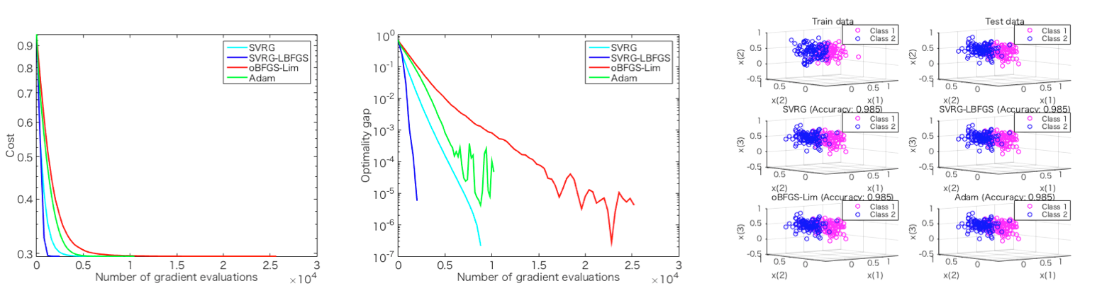
- Adam
- D. Kingma and J. Ba, "Adam: A method for stochastic optimization," International Conference for Learning Representation (ICLR), 2015.
- AdaMax
- D. Kingma and J. Ba, "Adam: A method for stochastic optimization," International Conference for Learning Representation (ICLR), 2015.
- Vanila SGD
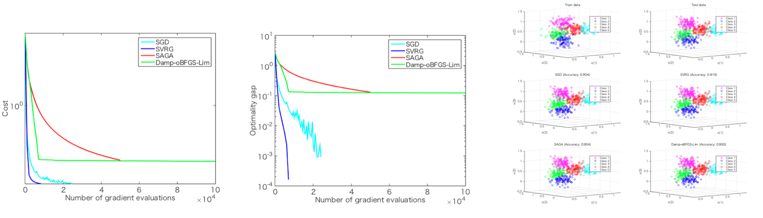
- Variance reduction variants
- SVRG (stochastic variance reduced gradient)
- R. Johnson and T. Zhang, "Accelerating stochastic gradient descent using predictive variance reduction," NIPS, 2013.
- SAG (stochastic average gradient)
- N. L. Roux, M. Schmidt, and F. R. Bach, "A stochastic gradient method with an exponential convergence rate for finite training sets," NIPS, 2012.
- SAGA
- A. Defazio, F. Bach, and S. Lacoste-Julien, "SAGA: A fast incremental gradient method with support for non-strongly convex composite objectives,", NIPS, 2014.
- SARAH (StochAstic Recusive gRadient algoritHm)
- L. M. Nguyen, J. Liu, K. Scheinberg, and M. Takac, "SARAH: A novel method for machine learning problems using stochastic recursive gradient," ICML, 2017.
- SVRG (stochastic variance reduced gradient)
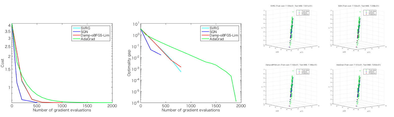
- Quasi-Newton variants
-
SQN (stochastic quasi-Newton)
- R. H. Byrd, ,S. L. Hansen J. Nocedal, and Y. Singer, "A stochastic quasi-Newton method for large-scale optimization," SIAM Journal on Optimization, vol. 26, Issue 2, pp. 1008-1031, 2016.
-
SVRG-SQN (denoted as "Stochastic L-BFGS" or "slbfgs" in the paper below.)
- P. Moritz, R. Nishihara and M. I. Jordan, "A linearly-convergent stochastic L-BFGS Algorithm," International Conference on Artificial Intelligence and Statistics (AISTATS), pp.249-258, 2016.
-
SVRG-LBFGS (denoted as "SVRG+II: LBFGS" in the paper below.)
- R. Kolte, M. Erdogdu and A. Ozgur, "Accelerating SVRG via second-order information," OPT2015, 2015.
-
SS-SVRG (denoted as "SVRG+I: Subsampled Hessian followed by SVT" in the paper below.)
- R. Kolte, M. Erdogdu and A. Ozgur, "Accelerating SVRG via second-order information," OPT2015, 2015.
-
oBFGS-Inf (Online BFGS, Infinite memory)
- N. N. Schraudolph, J. Yu and Simon Gunter, "A stochastic quasi-Newton method for online convex optimization ," International Conference on Artificial Intelligence and Statistics (AISTATS), pp.436-443, Journal of Machine Learning Research, 2007.
-
oLBFGS-Lim (Online BFGS, Limited memory)
-
N. N. Schraudolph, J. Yu and S. Gunter, "A stochastic quasi-Newton method for online convex optimization ," International Conference on Artificial Intelligence and Statistics (AISTATS), pp.436-443, Journal of Machine Learning Research, 2007.
-
A. Mokhtari and A. Ribeiro, "Global convergence of online limited memory BFGS," Journal of Machine Learning Research, 16, pp. 3151-3181, 2015.
-
-
Reg-oBFGS-Inf (Regularized oBFGS, Infinite memory) (denoted as "RES" in the paper below.)
- A. Mokhtari and A. Ribeiro, "RES: Regularized stochastic BFGS algorithm," IEEE Transactions on Signal Processing, vol. 62, no. 23, pp. 6089-6104, Dec., 2014.
-
Damp-oBFGS-Inf (Regularized damped oBFGS, Infinite memory) (denoted as "SDBFGS" in the paper below.)
- X. Wang, S. Ma, D. Goldfarb and W. Liu, "Stochastic quasi-Newton methods for nonconvex stochastic optimization," arXiv preprint arXiv:1607.01231, 2016.
-
IQN (incremental Quasi-Newton method)
- A. Mokhtari, M. Eisen and A. Ribeiro, "An Incremental Quasi-Newton Method with a Local Superlinear Convergence Rate," ICASSP2017, 2017.
-
- Inexact Hessian variants
- SCR (Sub-sampled Cubic Regularization)
- J. M. Kohler and A. Lucchi, "Sub-sampled Cubic Regularization for non-convex optimization," ICML, 2017.
- Sub-sampled TR (trust region)
- A. R. Conn, N. I. Gould and P. L. Toint, "Trust region methods," MOS-SIAM Series on Optimization, 2000.
- SCR (Sub-sampled Cubic Regularization)
- Else
- SVRG-BB (stochastic variance reduced gradient with Barzilai-Borwein)
- C. Tan, S. Ma, Y. Dai, Y. Qian, "Barzilai-Borwein step size for stochastic gradient descent," NIPS, 2016.
- SVRG-BB (stochastic variance reduced gradient with Barzilai-Borwein)
| Algorithm name in example codes | function | options.sub_mode |
other options |
|---|---|---|---|
| SGD | sgd |
||
| SGD-CM | sgd_cm |
'CM' |
|
| SGD-CM-NAG | sgd_cm |
'CM-NAG' |
|
| AdaGrad | adagrad |
'AdaGrad' |
|
| RMSProp | adagrad |
'RMSProp' |
|
| AdaDelta | adagrad |
'AdaDelta' |
|
| Adam | adam |
'Adam' |
|
| AdaMax | adam |
'AdaMax' |
|
| SVRG | svrg |
||
| SAG | sag |
'SAG' |
|
| SAGA | sag |
'SAGA' |
|
| SARAH | sarah |
||
| SQN | slbfgs |
'SQN' |
|
| SVRG-SQN | slbfgs |
'SVRG-SQN' |
|
| SVRG-LBFGS | slbfgs |
'SVRG-LBFGS' |
|
| SS-SVRG | subsamp_svrg |
||
| oBFGS-Inf | obfgs |
'Inf-mem' |
|
| oLBFGS-Lim | obfgs |
'Lim-mem' |
|
| Reg-oBFGS-Inf | obfgs |
'Inf-mem' |
regularized=true |
| Damp-oBFGS-Inf | obfgs |
'Inf-mem' |
regularized=true & damped=true |
| IQN | iqn |
||
| SCR | scr |
gradient_sampling=1 & Hessian_sampling=1 |
|
| Subsampled-TR | subsamp_tr |
gradient_sampling=1 & Hessian_sampling=1 |
|
| SVRG-BB | svrg_bb |
- Note that other algorithms could be configurable by selecting other combinations of sub_mode and options.
- L2-norm regularized multidimensional linear regression
- L2-norm regularized linear SVM
- L2-norm regularized logistic regression
- Softmax classification (multinomial logistic regression)
- Note that softmax classification problem does not support Hessian-vector product type algorithms, i.e., SQN, SVRG-SQN and SVRG-LBFGS.
- L1-norm regularized multidimensional linear regression
- L1-norm regularized logistic regression
- Sum quadratic problem
Additionally, the following problems are provided for gradient descent algorithms.
- Rosenbrock problem
- Quadratic problem
- General problem
./                      - Top directory.
./README.md             - This readme file.
./run_me_first.m        - The scipt that you need to run first.
./demo.m                - Demonstration script to check and understand this package easily.
|plotter/               - Contains plotting tools to show convergence results and various plots.
|tool/                  - Some auxiliary tools for this project.
|problem/               - Problem definition files to be solved.
|sgd_solver/            - Contains various stochastic optimization algorithms.
|sgd_test/              - Some helpful test scripts to use this package.
|gd_solver/             - Contains various gradient descent optimization algorithms.
|gd_test/               - Some helpful test scripts using gradient descent algorithms to use this package.
Run run_me_first for path configurations.
%% First run the setup script
run_me_first; Just execute demo for the simplest demonstration of this package. This is the case of logistic regression problem.
%% Execute the demonstration script
demo;
The "demo.m" file contains below.
%% generate synthetic data
% set number of dimensions
d = 3;
% set number of samples
n = 300;
% generate data
data = logistic_regression_data_generator(n, d);
%% define problem definitions
problem = logistic_regression(data.x_train, data.y_train, data.x_test, data.y_test);
%% perform algorithms SGD and SVRG
options.w_init = data.w_init;
options.step_init = 0.01;
[w_sgd, info_sgd] = sgd(problem, options);
[w_svrg, info_svrg] = svrg(problem, options);
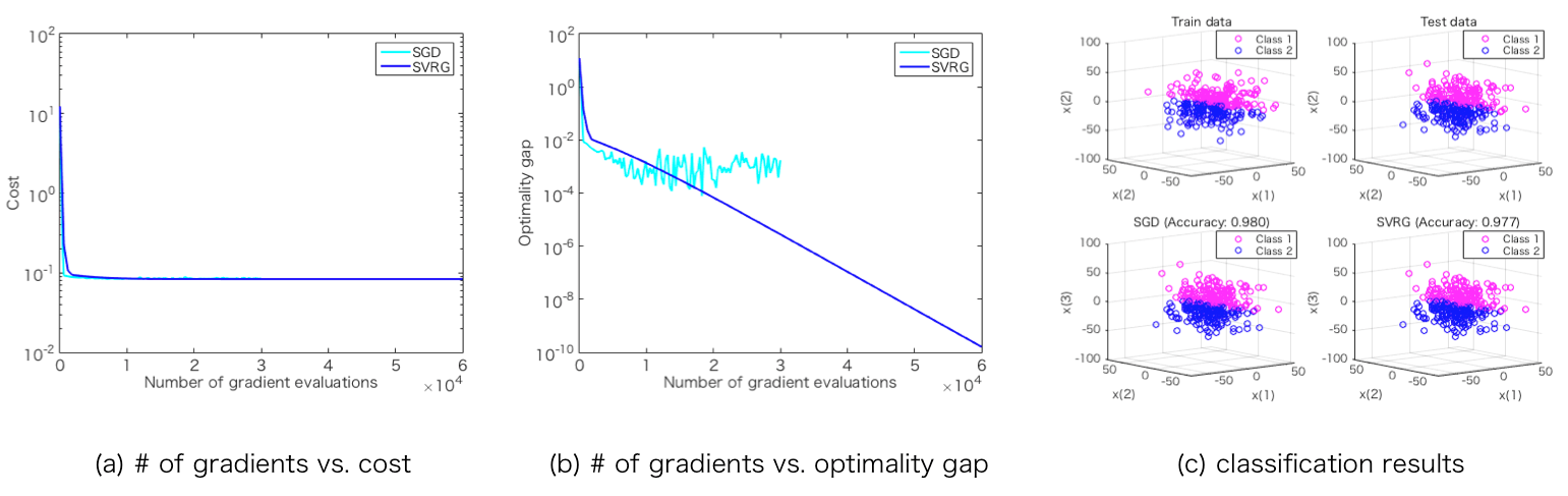
%% display cost/optimality gap vs number of gradient evaluations
display_graph('grad_calc_count','cost', {'SGD', 'SVRG'}, {w_sgd, w_svrg}, {info_sgd, info_svrg});
Let take a closer look at the code above bit by bit. The procedure has only **4 steps**!
Step 1: Generate data
First, we generate datasets including train set and test set using a data generator function logistic_regression_data_generator().
The output include train set and test set and an initial value of the solution w.
d = 3;
n = 300;
data = logistic_regression_data_generator(n, d);
Step 2: Define problem
The problem to be solved should be defined properly from the supported problems. logistic_regression() provides the comprehensive
functions for a logistic regression problem. This returns the cost value by cost(w), the gradient by grad(w) and the hessian by hess(w) when given w.
These are essential for any gradient descent algorithms.
problem = logistic_regression(data.x_train, data.y_train, data.x_test, data.y_test); Step 3: Perform solver
Now, you can perform optimization solvers, i.e., SGD and SVRG, calling solver functions, i.e., sgd() function and svrg() function after setting some optimization options.
options.w_init = data.w_init;
options.step_init = 0.01;
[w_sgd, info_sgd] = sgd(problem, options);
[w_svrg, info_svrg] = svrg(problem, options);
They return the final solutions of w and the statistics information that include the histories of epoch numbers, cost values, norms of gradient, the number of gradient evaluations and so on.
Step 4: Show result
Finally, display_graph() provides output results of decreasing behavior of the cost values in terms of the number of gradient evaluations.
Note that each algorithm needs different number of evaluations of samples in each epoch. Therefore, it is common to use this number to evaluate stochastic optimization algorithms instead of the number of iterations.
display_graph('grad_calc_count','cost', {'SGD', 'SVRG'}, {w_sgd, w_svrg}, {info_sgd, info_svrg});That's it!
"demo_ext.m" gives you more plots.
- Demonstration of "optimality gap"
For the calculation of "optimality gap", you need optimal solution w_opt beforehand by calling calc_solution() function of the problem definition function.
%% calculate optimal solution for optimality gap
w_opt = problem.calc_solution(1000);
options.f_opt = problem.cost(w_opt);
This case uses the full gradient descent solve gd() to obtain an optimal solution under max iteration 1000 with very precise tolerant stopping condition.
Then, you obtain the result of optimality gap by display_graph().
display_graph('grad_calc_count','optimality_gap', {'SGD', 'SVRG'}, {w_sgd, w_svrg}, {info_sgd, info_svrg}); - Demonstration of "classification accuracy"
Additionally, in this case of logistic regression, the results of classification accuracy are calculated using the corresponding prediction function prediction() and accuracy of the problem definition function logistic_regression().
Furthermore, the classification accuracies are illustrated by display_classification_result() function that is written in "demo.m" like below;
%% calculate classification accuracy
% for SGD
% predict
y_pred_sgd = problem.prediction(w_sgd);
% calculate accuracy
accuracy_sgd = problem.accuracy(y_pred_sgd);
fprintf('Classificaiton accuracy: %s: %.4f\n', 'SGD', accuracy_sgd);
% convert from {1,-1} to {1,2}
y_pred_sgd(y_pred_sgd==-1) = 2;
y_pred_sgd(y_pred_sgd==1) = 1;

% for SVRG
% predict
y_pred_svrg = problem.prediction(w_svrg);
% calculate accuracy
accuracy_svrg = problem.accuracy(y_pred_svrg);
fprintf('Classificaiton accuracy: %s: %.4f\n', 'SVRG', accuracy_svrg);
% convert from {1,-1} to {1,2}
y_pred_svrg(y_pred_svrg==-1) = 2;
y_pred_svrg(y_pred_svrg==1) = 1;


%% display classification results
% convert from {1,-1} to {1,2}
data.y_train(data.y_train==-1) = 2;
data.y_train(data.y_train==1) = 1;
data.y_test(data.y_test==-1) = 2;
data.y_test(data.y_test==1) = 1;
% display results
display_classification_result(problem, {'SGD', 'SVRG'}, {w_sgd, w_svrg}, {y_pred_sgd, y_pred_svrg}, {accuracy_sgd, accuracy_svrg}, data.x_train, data.y_train, data.x_test, data.y_test);
Output results:
- Demonstration of "convergence animation"
You need specify additional options before executing solvers.
%% set options for convergence animation
options.max_epoch = 100;
options.store_w = true;
Then, draw_convergence_animation() draws a convergence animation. Note that draw_convergence_animation() is executable when only the dimension of the parameters is 2.
%% display convergence animation
draw_convergence_animation(problem, {'SGD', 'SVRG'}, {info_sgd.w, info_svrg.w}, options.max_epoch); - Linear regression problem
- Softmax classifier problem
- Linear SVM problem
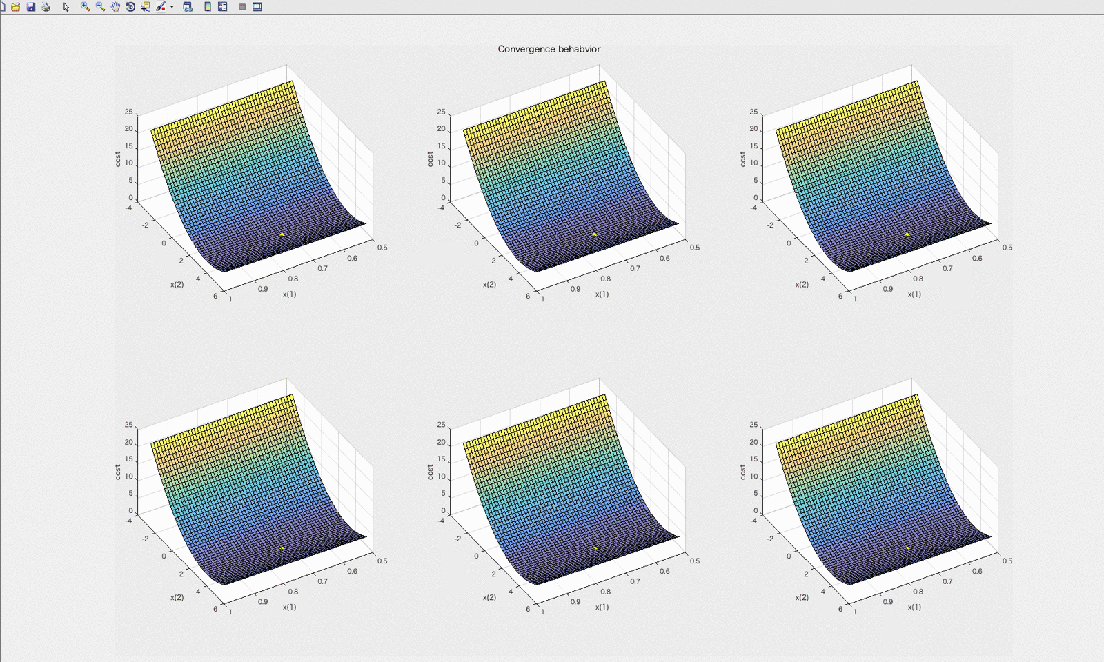
"test_convergence_animation_demo.m" provides you an animation of convergence behaviors of algorithms. Please click the image below to see its animation.
- The SGDLibrary is free and open source.
- The code provided iin SGDLibrary should only be used for academic/research purposes.
- The codes provided by original papers are included. (Big thanks !!!)
- iqn.m: originally created by A. Mokhtari.
- The codes ported from original python codes are included. (Big thanks !!!)
- scr.m, cr_subsolver.m, subsamp_tr.m, tr_subsolver.m: Python codes are originally created by J. M. Kohler and A. Lucchi. These MATLAB codes are ported with original authors' big helps.
- Third party files are included.
- subsamp_newton.m: originally created by Peng Xu and Jiyan Yang in Subsampled-Newton. This is modifided to handle other problems like linear regression.
- Proximal Solver from FOM
- As always, parameters such as the step size should be configured properly in each algorithm and each problem.
- Softmax classification problem does not support "Hessian-vector product" type algorithms, i.e., SQN, SVRG-SQN and SVRG-LBFGS.
- This SGDLibrary internally contains the GDLibrary.
If you have any problems or questions, please contact the author: Hiroyuki Kasai (email: hiroyuki dot kasai at waseda dot jp)
- Version 1.0.20 (Nov. 10, 2020)
- Buf fixed, and some files are added.
- Version 1.0.19 (Oct. 27, 2020)
- Buf fixed, and some files are added.
- Version 1.0.17 (Apr. 17, 2018)
- Sub-sampled CR (including ARC) and Sub-sampled TR are nely added.
- Version 1.0.16 (Apr. 01, 2018)
- GNU Octave is supported.
- Change the functions of problem into class-based definitions.
- Version 1.0.12 (Sep. 29, 2017)
- SARAH is nely added.
- Version 1.0.11 (Sep. 28, 2017)
- SGD-CM and SGD-CM-NAG are nely added.
- Version 1.0.10 (Sep. 26, 2017)
- Options paramter in solvers is re-organized.
- Separate the function to store statistics information from solver.
- Version 1.0.9 (Sep. 25, 2017)
- Proximal operator is newly added.
- Some new problems are added.
- User-defined stepsize algorithm is supported. See test_stepsize_alg_demo.m.
- Version 1.0.8 (Mar. 28, 2017)
- IQN (incremental Quasi-Newton method, iqn.m) is nely included.
- Version 1.0.7 (Mar. 17, 2017)
- Add some functions and modify items.
- Version 1.0.6 (Mar. 13, 2017)
- Add some functions and modify items. Sum quadratic problem is added.
- Version 1.0.5 (Jan. 12, 2017)
- Add some functions and modify items.
- Version 1.0.4 (Nov. 04, 2016)
- Integrate GDLibrary with SGDLibrary.
- Version 1.0.3 (Nov. 04, 2016)
- Modify many items.
- Version 1.0.2 (Nov. 01, 2016)
- SVRG-BB (SVRG with Barzilai-Borwein) is added.
- Version 1.0.1 (Oct. 28, 2016)
- SS-SVRG (Subsampled Hessian algorithm followed by SVT) is added.
- Convergence behavior animation function is added.
- Version 1.0.0 (Oct. 27, 2016)
- Initial version.


