bifurcationkit / bifurcationkit.jl Goto Github PK
View Code? Open in Web Editor NEWA Julia package to perform Bifurcation Analysis
Home Page: https://bifurcationkit.github.io/BifurcationKitDocs.jl/stable
License: Other
A Julia package to perform Bifurcation Analysis
Home Page: https://bifurcationkit.github.io/BifurcationKitDocs.jl/stable
License: Other


Hello,
I have a 2 variable ODE system for which I want to computer a bifurcation diagram. I managed to get a sketch of it on previous versions:

The paths didn't manage to track all of the ways properly, but it seems to have a single steady state, then a region with 5, then a region with 3, then 5 and then 1 again. I think there are 2 branch points and 4 fold points.
I managed to get that sketch using deflated continuation, but I think the code don't work anymore, and it looked kind of weird, so I figured maybe I should try using the bifurcation diagram feature (https://rveltz.github.io/BifurcationKit.jl/dev/BifurcationDiagram/) which computes it recursively (but then that might have some problems because there's a cycle). Possibly branch switching is better (https://rveltz.github.io/BifurcationKit.jl/dev/branchswitching/), since I know more or less what to expect.
However, all of the inputs for these methods require the function and 3 derivatives. Because I get my function via reaction networks I have the function, and the first derivative (the Jacobian, but that is what is being requested, right). Is it possible to perform these with only those two inputs (I tried, but got some error, but it might be I am making some other input mistake). Is there any disadvantage to not providing 2nd and 3rd derivatives?
Hi, great package!
I'm trying to make a Hopf continuation for a simple ODE system:
function simpleSystem!(dx, x, p, t)
	@unpack B, β, Da = p
	x1, x2 = x
	dx[1] = -x1 + Da*(1-x1)*exp(x2)
	dx[2] =	-x2 + B*Da*(1-x1)*exp(x2)-β*(x2)
	dx
end

simpleSystem(x, p) = simpleSystem!(similar(x), x, p, 0)
jet  = BK.getJet(simpleSystem; matrixfree=false)

par_simpleSystem = (B=7.06, β=0.74, Da=0.15)
x0 = [0.4,0.4]

opts_br = ContinuationPar(pMin = 0.13, pMax = 0.16	, ds = -0.001, dsmax = 0.01, nInversion = 20,
	detectBifurcation = 3, maxBisectionSteps = 8, nev = 30, plotEveryStep = 20, maxSteps = 1500,
	theta = 0.03)

br, = continuation(jet[1], jet[2], x0, par_firstOrder, (@lens _.Da), opts_br;
	recordFromSolution = recordFromSolution,
	#bothside = true,
	plot = false, verbosity = 0, normC = norminf)

scene = plot(br)
The branch should be correct, but my Hopf continuation on the two Hopf points failed.
Could you tell me how to get the Hopf continuation work?
Hi,
When trying to use Multiple Poincare Shooting, I get the following error. Maybe @ChrisRackauckas has an idea...
julia> res = @time probMPsh(par_hopf)(initpo, initpo)
ERROR: Event repeated at the same time. Please report this error
Stacktrace:
 [1] apply_callback!(::OrdinaryDiffEq.ODEIntegrator{Tsit5,false,Array{Float64,1},Float64,NamedTuple{(:r, :μ, :ν, :c3, :c5),NTuple{5,Float64}},Float64,Float64,Float64,Array{Array{Float64,1},1},ODESolution{Float64,2,Array{Array{Float64,1},1},Nothing,Nothing,Array{Float64,1},Array{Array{Array{Float64,1},1},1},ODEProblem{SubArray{Float64,1,Array{Float64,2},Tuple{Base.Slice{Base.OneTo{Int64}},Int64},true},Tuple{Float64,Float64},false,NamedTuple{(:r, :μ, :ν, :c3, :c5),NTuple{5,Float64}},ODEFunction{false,typeof(Fsl),UniformScaling{Bool},Nothing,Nothing,Nothing,Nothing,Nothing,Nothing,Nothing,Nothing,Nothing,Nothing,Nothing},Base.Iterators.Pairs{Union{},Union{},Tuple{},NamedTuple{(),Tuple{}}},DiffEqBase.StandardODEProblem},Tsit5,OrdinaryDiffEq.InterpolationData{ODEFunction{false,typeof(Fsl),UniformScaling{Bool},Nothing,Nothing,Nothing,Nothing,Nothing,Nothing,Nothing,Nothing,Nothing,Nothing,Nothing},Array{Array{Float64,1},1},Array{Float64,1},Array{Array{Array{Float64,1},1},1},OrdinaryDiffEq.Tsit5ConstantCache{Float64,Float64}},DiffEqBase.DEStats},ODEFunction{false,typeof(Fsl),UniformScaling{Bool},Nothing,Nothing,Nothing,Nothing,Nothing,Nothing,Nothing,Nothing,Nothing,Nothing,Nothing},OrdinaryDiffEq.Tsit5ConstantCache{Float64,Float64},OrdinaryDiffEq.DEOptions{Float64,Float64,Float64,Float64,typeof(DiffEqBase.ODE_DEFAULT_NORM),typeof(opnorm),CallbackSet{Tuple{VectorContinuousCallback{PseudoArcLengthContinuation.var"#pSection#599"{typeof(section!)},PseudoArcLengthContinuation.var"#affect!#600",Nothing,typeof(DiffEqBase.INITIALIZE_DEFAULT),Float64,Int64,Nothing}},Tuple{}},typeof(DiffEqBase.ODE_DEFAULT_ISOUTOFDOMAIN),typeof(DiffEqBase.ODE_DEFAULT_PROG_MESSAGE),typeof(DiffEqBase.ODE_DEFAULT_UNSTABLE_CHECK),DataStructures.BinaryHeap{Float64,DataStructures.LessThan},DataStructures.BinaryHeap{Float64,DataStructures.LessThan},Nothing,Nothing,Int64,Array{Float64,1},Array{Float64,1},Array{Float64,1}},Array{Float64,1},Float64,DiffEqBase.CallbackCache{Array{Float64,N} where N,Array{Float64,N} where N}}, ::VectorContinuousCallback{PseudoArcLengthContinuation.var"#pSection#599"{typeof(section!)},PseudoArcLengthContinuation.var"#affect!#600",Nothing,typeof(DiffEqBase.INITIALIZE_DEFAULT),Float64,Int64,Nothing}, ::Float64, ::Float64, ::Int64) at /Users/rveltz/.julia/packages/DiffEqBase/YIwj5/src/callbacks.jl:667
The example is as follows:
using DifferentialEquations, DiffEqOperators, ForwardDiff
	using PseudoArcLengthContinuation, LinearAlgebra, Parameters, Setfield
	const PALC = PseudoArcLengthContinuation

norminf = x -> norm(x, Inf)
function Fsl!(f, u, p)
	@unpack r, μ, ν, c3, c5 = p
	u1 = u[1]
	u2 = u[2]

	ua = u1^2 + u2^2

	f[1] = r * u1 - ν * u2 - ua * (c3 * u1 - μ * u2) - c5 * ua^2 * u1
	f[2] = r * u2 + ν * u1 - ua * (c3 * u2 + μ * u1) - c5 * ua^2 * u2

	return f
end

function Fsl(x, p, t)
	f = similar(x)
	Fsl!(f, x, p)
end

Fode(f, x, p, t) = Fsl!(f, x, p)
Jsl(x, dx, p) = ForwardDiff.derivative(t -> Fsl(x .+ t .* dx, p), 0.)
# JacOde(J, x, p, t) = copyto!(J, Jsl(x, p))

par_sl = (r = 0.5, μ = 0., ν = 1.0, c3 = 1.0, c5 = 0.0,)
u0 = [.001, .001]

par_hopf = (@set par_sl.r = 0.1)
probsundials = ODEProblem(Fsl, u0, (0., 100.), par_hopf)

function section!(out, x)
	M = 4
	for ii=1:M
		th = 2pi*ii/M
		tmp = [-sin(th), cos(th)]
		out[ii] = dot(x, tmp)
	end
	out
end

# standard simple shooting
M = 4
probMPsh = p -> PALC.PoincareShootingProblem(u -> Fsl(u, p, 0.), p, probsundials, Tsit5(), M, section!; atol = 1e-10, rtol = 1e-9)

r = 1.04

initpo = Float64[]
for ii=1:M
	th = 2pi*ii/M
	push!(initpo, r*cos(th))
	push!(initpo, r*sin(th))

end

res = @time probMPsh(par_hopf)(initpo);
norminf(res)
# 0.005197 seconds (61.15 k allocations: 4.358 MiB)
# 0.4953547991423255
however, this returns an error:
res = @time probMPsh(par_hopf)(initpo, initpo);
Right now, only GLMakie backend is allowed, for e.g. WGLMakie or CairoMakie, RecipesMakie.jl is not loaded (as per this line)
Also, RecipesMakie.jl seems to only support GLMakie (but that's only my assumption).
Thanks a lot
I have a problem that p is strictly constrained in a range, say [a, b], (which can be computed). When p is out of this range, the evaluation of the function will fail. In my case, a negative will be given to the log function. Currently, when I set pMin=a+eps(), and pMax=b-eps(), the parameter prediction step will still predict a value outside the range [a, b], which leads to the failing of the whole continuation process.
Sample output is
      From worker 2:	Continuation Step 339
      From worker 2:	Step size = 2.0000e-03
      From worker 2:	Parameter Aα = 8.2503e-01 ⟶  8.2741e-01 [guess]
      From worker 2:	--> Step Converged in 2 Nonlinear Iteration(s)
      From worker 2:	Parameter Aα = 8.2503e-01 ⟶  8.2741e-01
      From worker 2:	Predictor: BifurcationKit.SecantPred()
      From worker 2:	--> Computed 3 eigenvalues in 1 iterations, #unstable = 3
      From worker 2:	──────────────────────────────────────────────────────────────────────
      From worker 2:	Continuation Step 340
      From worker 2:	Step size = 2.0000e-03
      From worker 2:	Parameter Aα = 8.2741e-01 ⟶  8.2979e-01 [guess]
For this problem, my b is 0.829285. As can be seen, the prediction of p in Step 340 is 0.82979 (>0.829285), which leads to the breaking of my continuation process.
I wonder if we can make the [pMin, pMax] constraint hard, so that p never goes outside of it. Or even better, BK can detect the failing of evaluation of the function when the prediction of p is outside the range, and reduce the step size accordingly to force the prediciton of p lies in the range.
Would be good to show users that its possible to use this library with DiffEqBiological
using DiffEqBiological,BifurcationKit
using Setfield,LinearAlgebra,Plots

system = @reaction_network begin
     k₁,		Y → 2X
     2k₂,		2X → X + Y
     k₃,		X + Y → Y
     k₄,		X → 0
end k₁ k₂ k₃ k₄

# get rate function and jacobian, for use in continuation
F! = oderhsfun(system)
function F(u::Vector{T},p::NamedTuple) where T<:Number
	f = similar(u)
	F!(f,u,[ p[key] for (key, value) ∈ paramsmap(system) ],Inf)
	return f
end

∂Fu! = jacfun(system)
function ∂Fu(u::Vector{T},p::NamedTuple) where T<:Number
	J = zeros(T,length(u),length(u))
	∂Fu!(J,u,[ p[key] for (key, value) ∈ paramsmap(system) ],Inf)
	return J
end

# define the parameter direction that you want to explore
pRange = range(0,12,length=200)
parameter_name = (@lens _.k₁)
p = (k₁=0.0, k₂=1.0, k₃=1.0, k₄=1.5)

# options for branch continuation along parameter direction
options = ContinuationPar( maxSteps = 5000,
	dsmax=10*step(pRange), dsmin=step(pRange), ds=step(pRange),
	pMin = minimum(pRange), pMax=maximum(pRange),
	newtonOptions = NewtonPar(tol = 1e-8),
	saveEigenvectors = false
)

# options for detecting multiple branches
deflation = DeflationOperator(2.0, dot, 1.0, [ zeros(length(species(system))) ])
termination_condition(x, f, J, residual, iteration, niter, options; kwargs...) = residual <1e3
root_search(x,p,id) = x .+ rand(length(x))

##################################### main continuation method
@assert( det(∂Fu(randn(length(species(system))),p)) ≠ 0, "species must be linearly independent")
branches, = continuation( F, ∂Fu, p, parameter_name, options, deflation; showplot=false,
	callbackN = termination_condition, perturbSolution = root_search )

#################################### display results
plot(size=(500,500),ylabel="steady states", xlabel="parameter $(first(typeof(parameter_name).parameters))")
plot!(branches,lw=3,label="")
Hello,
I am following the instructions under https://rveltz.github.io/PseudoArcLengthContinuation.jl/dev/iterator/ to make a bifurcation diagram of a system I am investigating. While I can get the base example to work by running it, I have problems making it work as I'd like for a more general system (and when it works, I am a bit uncertain why).
In the example, I am using DiffEqBiological to generate a model, from which I then generate the system function and jacobian. The model equation is
dX/dt = v0 + v*(X^n)/(K^n + X^n) - d*X
and I want to plot the value of the system's fixed point(s) as the parameter v varies from 0.1 to 5.0.
Please see the following code:
# Fetch stuff
using PseudoArcLengthContinuation, SparseArrays, LinearAlgebra, Plots, Setfield, UnPack
const PALC = PseudoArcLengthContinuation
using DiffEqBiological # Required to generate my system

# Taken from the docs. Don't know why we are doing this.
normInf = x -> norm(x, Inf)

# Generates my functions
# A reactio network. This generates the stuff for a model system with a single variable and 5 parameters.
rn = @reaction_network begin
	v0+hill(X,v,K,n), 0 --> X
	d, X --> 0
end v0 v K n d

# The reaction network structures contain the right functions, however, they are designed for DifferentialEquations and requires modification.
# The original functions do not return the output, but rather modifes an input vector/matrix with the desired values. Also, the parameters works differently (I tried it the natural way, ran into problems, but I will worry about that when I got the main methodology working).
function F(x,p)
	@unpack v0,v,K,n,d = p
	output = copy(x)
	rn.f(output,x,[v0, v, K, n, d],0.)
	return output
end
function J(x,p)
	@unpack v0,v,K,n,d = p
	output = zeros(length(x),length(x))
	rn.jac(output,x,[v0, v, K, n, d],0.)
	return output
end

# Just taken from the docs. I modified pMin and pMax to 0.1 and 10.0. I sat pMin to 0.1 because that was my best guess at the initial value.
opts = PALC.ContinuationPar(dsmax = 0.1, dsmin = 1e-5, ds = -0.001, maxSteps = 130, pMin = 0.1, pMax = 10.0, saveSolEveryNsteps = 0, computeEigenValues = true, detectBifurcation = true, newtonOptions = NewtonPar(tol = 1e-8, verbose = true))

# Set the parameters. I sat v to 5. because I thought that might be the final value.
pars = (v0=0.1, v=5., K=0.5, n=3., d=1.2)

# Tries to define the iterator. The fixed point of the system for v=0.1 is 0.08333333333333334.
iter = PALC.PALCIterable(F, J, [0.08333333333333334], pars, (@lens _.v), opts; verbosity = 2)

# This is just taken directly from the example.
resp = Float64[]
resx = Float64[]
for state in iter
	push!(resx, getx(state)[1])
	push!(resp, getp(state))
end

#This plot
plot(resp, resx; label = "", xlabel = "v")
Now, this plot gets rather "jagged", and I'd like it smoother. I try setting
opts = PALC.ContinuationPar(dsmax = 0.01, dsmin = 1e-3, ds = -0.001, maxSteps = 1300,...
but this makes the end result weird. I try modifying ds = 0.001, but that makes things worse. What should I do here?
Also, could someone confirm how I set the initial and final values of the parameter, as well as exactly where I should make my initial x0 guess? I got it right here, but I would like to be sure why I am right.
Looking forward to getting this working!
Cheers
Hi, every example I have tried to run crashes Julia 1.4.1 on my machine.
In the chan.jl example, this occurs on line 76, or skipping the call to newton, on line 82. Likewise, the script crashes on lines 92 or 101 if the previous crashing calls are skipped.
Some of the crash message:
julia> outfold, _, flag = @time newton(
               F_chan, Jac_mat,
               #index of the fold point
               br, indfold, par, (@lens _.α))
Illegal inttoptr
	  %90 = ptrtoint double addrspace(13)* %88 to i64
Illegal inttoptr
	  %scevgep3536 = ptrtoint double addrspace(13)* %scevgep35 to i64
Illegal inttoptr
	  %100 = inttoptr i64 %99 to i8 addrspace(13)*

signal (6): Aborted
in expression starting at REPL[27]:1
gsignal at /usr/bin/../lib/x86_64-linux-gnu/libc.so.6 (unknown line)
abort at /usr/bin/../lib/x86_64-linux-gnu/libc.so.6 (unknown line)
unknown function (ip: 0x7f3242ef3d04)
Apologies if that isn't helpful; I'm just not sure how to track down the underlying issue.
The matrix-free portion of the example runs without issue (starting from line 108).
Dear authors,
I was following the plotting examples from #27, but was not sure whether there is support for NonLinearProblem. Specifically, I am trying to train a neural network (deep equilibrium models) using the NonLinearProblem wrapper, and it is not clear to me what parameters I should pass into continuation. When I run the following function, this error occurs (any help would be appreciated, especially references to visualization of NonLinearProblems)---
ann = Chain(Dense(1, 2), Dense(2, 1))
p,re = Flux.destructure(ann)
pRange = (0.1,20.)

function solve_ss(x)
    z = re(p)(x)
    function dudt_(u, _p)
        re(_p)(u+x) - u
    end

    ss = NonlinearProblem{false}(dudt_, z, p)
    x = solve(ss, NewtonRaphson(), tol = 1f-5)#.u
    options = ContinuationPar( maxSteps=50000,
        dsmax=(pRange[2]-pRange[1])*1e-3, dsmin=(pRange[2]-pRange[1])*1e-9, ds=(pRange[2]-pRange[1])*1e-9,
        pMin=pRange[1], pMax=pRange[2], detectBifurcation=1,
        newtonOptions = NewtonPar(tol = 1e-8, verbose = false));
    path = continuation((u,p)->fun(u,p,0), (u,p)->fun.jac(u,p,0), z, (@lens _.p), options; tangentAlgo=BorderedPred());
    plot(path[1],grid=false,xguide="$p",plotfold=false,label="",framestyle=:box)
end
ERROR: LoadError: type Array has no field p
Stacktrace:
[1] getproperty(x::Vector{Float32}, f::Symbol)
@ Base ./Base.jl:33
[2] get(obj::Vector{Float32}, l::Setfield.PropertyLens{:p})
@ Setfield ~/.julia/packages/Setfield/NshXm/src/lens.jl:105
[3] iterate(it::ContIterable{var"#61#64", BifurcationKit.var"#143#145"{var"#61#64"}, var"#62#65", Vector{Float32}, Setfield.PropertyLens{:p}, Float64, DefaultLS, DefaultEig{typeof(real)}, BorderedPred, BorderingBLS{DefaultLS, Float64}, BifurcationKit.var"#118#128"{BifurcationKit.var"#118#119#129"}, BifurcationKit.var"#120#130"{BifurcationKit.var"#120#121#131"}, typeof(norm), BifurcationKit.DotTheta{BifurcationKit.var"#122#132"}, typeof(BifurcationKit.finaliseDefault), typeof(BifurcationKit.cbDefault), Nothing, String}; _verbosity::Int64)
@ BifurcationKit ~/.julia/packages/BifurcationKit/Yvq7p/src/Continuation.jl:244
[4] iterate(it::ContIterable{var"#61#64", BifurcationKit.var"#143#145"{var"#61#64"}, var"#62#65", Vector{Float32}, Setfield.PropertyLens{:p}, Float64, DefaultLS, DefaultEig{typeof(real)}, BorderedPred, BorderingBLS{DefaultLS, Float64}, BifurcationKit.var"#118#128"{BifurcationKit.var"#118#119#129"}, BifurcationKit.var"#120#130"{BifurcationKit.var"#120#121#131"}, typeof(norm), BifurcationKit.DotTheta{BifurcationKit.var"#122#132"}, typeof(BifurcationKit.finaliseDefault), typeof(BifurcationKit.cbDefault), Nothing, String})
@ BifurcationKit ~/.julia/packages/BifurcationKit/Yvq7p/src/Continuation.jl:243
[5] continuation(it::ContIterable{var"#61#64", BifurcationKit.var"#143#145"{var"#61#64"}, var"#62#65", Vector{Float32}, Setfield.PropertyLens{:p}, Float64, DefaultLS, DefaultEig{typeof(real)}, BorderedPred, BorderingBLS{DefaultLS, Float64}, BifurcationKit.var"#118#128"{BifurcationKit.var"#118#119#129"}, BifurcationKit.var"#120#130"{BifurcationKit.var"#120#121#131"}, typeof(norm), BifurcationKit.DotTheta{BifurcationKit.var"#122#132"}, typeof(BifurcationKit.finaliseDefault), typeof(BifurcationKit.cbDefault), Nothing, String})
@ BifurcationKit ~/.julia/packages/BifurcationKit/Yvq7p/src/Continuation.jl:458
[6] continuation(Fhandle::Function, Jhandle::Function, x0::Function, par::Vector{Float32}, lens::Setfield.PropertyLens{:p}, contParams::ContinuationPar{Float64, DefaultLS, DefaultEig{typeof(real)}}, linearAlgo::BorderingBLS{DefaultLS, Float64}; bothside::Bool, kwargs::Base.Iterators.Pairs{Symbol, BorderedPred, Tuple{Symbol}, NamedTuple{(:tangentAlgo,), Tuple{BorderedPred}}})
@ BifurcationKit ~/.julia/packages/BifurcationKit/Yvq7p/src/Continuation.jl:0
[7] continuation(Fhandle::Function, Jhandle::Function, x0::Function, par::Vector{Float32}, lens::Setfield.PropertyLens{:p}, contParams::ContinuationPar{Float64, DefaultLS, DefaultEig{typeof(real)}}; linearAlgo::Nothing, kwargs::Base.Iterators.Pairs{Symbol, BorderedPred, Tuple{Symbol}, NamedTuple{(:tangentAlgo,), Tuple{BorderedPred}}})
@ BifurcationKit ~/.julia/packages/BifurcationKit/Yvq7p/src/Continuation.jl:591
[8] continuation(Fhandle::var"#61#64", x0::Function, par::Vector{Float32}, lens::Setfield.PropertyLens{:p}, contParams::ContinuationPar{Float64, DefaultLS, DefaultEig{typeof(real)}}; kwargs::Base.Iterators.Pairs{Symbol, BorderedPred, Tuple{Symbol}, NamedTuple{(:tangentAlgo,), Tuple{BorderedPred}}})
@ BifurcationKit ~/.julia/packages/BifurcationKit/Yvq7p/src/Continuation.jl:594
[9] solve_ss(x::Vector{Int64})
@ Main ~/julia/simpleDEQ.jl:37
[10] top-level scope
@ ~/julia/simpleDEQ.jl:62
[11] include(fname::String)
@ Base.MainInclude ./client.jl:444
[12] top-level scope
@ none:1
in expression starting at /Users/qiyaowei/julia/simpleDEQ.jl:62
I am using the bifurcationdiagram on a simple function (with a bistable region. However, there is a weird jump in the diagram (best just seen in the image at the end). It seems something weird gets mixed up.
# Fetch packages
using ModelingToolkit, OrdinaryDiffEq, BifurcationKit, Plots, Setfield, LinearAlgebra

# Declare model.
@parameters t s d T v0 n
@variables X(t) A1(t) A2(t) A3(t)
D = Differential(t)

eqs = [D(X) ~ v0 + ((s*X)^n)/((s*X)^n + (d*A3)^n + 1) - X,
       D(A1) ~ (X-A1)/T,
       D(A2) ~ (A1-A2)/T,
       D(A3) ~ (A2-A3)/T]

@named sys = ODESystem(eqs);

# Prepares input
params_input = [0.25,1.0,0.1,3,0.1]  # Order is "d,s,v0,n,T", check in "sys.ps". Should be fine.
p_span = (1.,4.);
#odefun = ODEFunction(convert(ODESystem,network),jac=true)
odefun = ODEFunction(sys,jac=true)
F = (u,p) -> odefun(u,p,0)
J = (u,p) -> odefun.jac(u,p,0)
jet = BifurcationKit.getJet(F, J; matrixfree=false)

u0 = solve(ODEProblem(sys,rand(length(sys.states)),(0.,100.0),params_input),Rosenbrock23()).u[end];

# Sets options
dsmax = 1e-2
dsmin = 1e-5
ds = sqrt(dsmax*dsmin);
maxSteps = 10000
opts_br = ContinuationPar(pMin = p_span[1], pMax = p_span[2], dsmax = dsmax, dsmin = dsmin, ds=ds, maxSteps=maxSteps,
detectBifurcation = 3, nInversion = 6, maxBisectionSteps = 25,nev = 4);

# Calculates the diagram.
bif = bifurcationdiagram(jet..., u0, params_input, (@lens _[2]), 2,
    (x,p,level)->setproperties(opts_br);
    tangentAlgo = SecantPred(),
    recordFromSolution=(x, p) -> x[1], verbosity = 0, plot=false);

# Plots the diagram.
plot(bif)
This is my Pkg.status()
  [0f109fa4] BifurcationKit v0.1.8
  [479239e8] Catalyst v10.2.0 `~/.julia/dev/Catalyst`
  [c894b116] DiffEqJump v8.0.0
  [0c46a032] DifferentialEquations v6.20.0
  [961ee093] ModelingToolkit v7.1.3
  [1dea7af3] OrdinaryDiffEq v5.69.0
  [91a5bcdd] Plots v1.24.3
  [f27b6e38] Polynomials v2.0.17
  [295af30f] Revise v3.2.0
  [2913bbd2] StatsBase v0.33.13
  [f3b207a7] StatsPlots v0.14.29
  [789caeaf] StochasticDiffEq v6.41.0
Thanks for the fantastic package. Briefly, I have some problems trying to find periodic orbits for a system built from Catalyst.jl for which I know a Hopf bifurcation.
I am unsure if the problem comes from building the system, a wrong choice of tolerance parameters or something else.
The system is the following.
using Catalyst, LinearAlgebra

rn = @reaction_network begin
    k1,  X2 → X1
    k2,  X1 → X2
    k3,  X3 → X5
    k4,  X5 → X4
    k5,  X4 → X6
    k6,  X4 → X3
    k7,  X6 → X5
    k8,  X1 + X5 → X2 + X3
    k9,  X1 + X6 → X2 + X4
end k1 k2 k3 k4 k5 k6 k7 k8 k9
Catalyst.reorder_states!(rn, [2,1,3,5,4,6])
The Hopf bifurcation occurs at
Xs = [1.6563516576558746, 3.5232975392793924e8, 1.0, 0.0038843824790898043, 3.7708607296986027e-10, 0.08021161610521155]
Ks = [2.8384448207706775e-9, 2.276606366932523e-10, 1.0000091094346868, 29473.54319518398, 0.01816749288551057, 0.002345143593835089, 2.499174147678733e-5, 1.6010576150026472e9, 0.0005160737862267585]
We can check that the system has nontrivial conservative laws
N = netstoichmat(rn)
W = conservationlaws(N)
So, for example, when we call continuation to compute a bifurcation diagram, we get a "singularity error".
To avoid this error, I build the smooth system as follows.
Question0 (provably for Catalyst.jl people): Does it sound reasonable to build the system in this way?
## Singular system
odesys = convert(ODESystem, rn; combinatoric_ratelaws=false)
odefun = ODEFunction(odesys; jac=true)

## Smooth system
# Conservative laws
states_new = states(rn)
Ts = W * Xs
states_new[2] = Ts[1] - states(rn)[1]
states_new[3] = Ts[2] - sum(states(rn)[4:6])

# Build the new system
odefun_new = odefun(states_new, parameters(rn), odesys.iv)
D = Differential(odesys.iv)
eqs_new = equations(odesys)

ind_new = [1,4,5,6]
eqs_new = [D(states(rn)[i]) ~ odefun_new[i] for i in ind_new]

@named odesys_smooth = ODESystem(
    eqs_new,
    odesys.iv,
    [states(rn)[i] for i in ind_new],
    parameters(rn))

odefun_smooth = ODEFunction(odesys_smooth; jac=true)
F_smooth(u, p) = odefun_smooth(u, p, 0.)
J_smooth(u, p) = odefun_smooth.jac(u, p, 0.)
## Sanity check
Xs_smooth = [Xs[i] for i in [1,4,5,6]]
F_smooth(Xs_smooth, Ks)
det(J_smooth(Xs_smooth, Ks))
Now, I want the bifurcation diagram for X4 w.r.t. parameter k9:
p_idx = 9                     # The index of the bifurcation parameter.
p_span = (0.000, 1.)   # The parameter range for the bifurcation diagram.
plot_var_idx = 4          # The index of the variable we plot in the bifurcation diagram.
# I know about the option `bothside=true`, but I am not sure how to use it, so first I track the solution `Xs` along `k9` using [HomotopyContinuation.jl.](https://github.com/JuliaHomotopyContinuation/HomotopyContinuation.jl)
import HomotopyContinuation
const HC = HomotopyContinuation

# Translate vars and params to HC
hc_vars = HC.Variable.(Symbol.([states(rn)[i] for i in ind_new]))
hc_params = Vector{Any}(undef, length(Ks))
hc_param = HC.Variable(Symbol(Catalyst.parameters(rn)[p_idx]))

# Set all parameters except `k9`, for which we want to track.
hc_params .= Ks
hc_params[p_idx] = hc_param

# Build HC.system with one parameter
hc_eqs_smooth = F_smooth(hc_vars, hc_params)
hc_sys_smooth = HC.System(hc_eqs_smooth; variables=hc_vars, parameters=[hc_param])

# Track `Xs` along `k9`
x₀ = HC.solve(hc_sys_smooth, Xs_smooth; start_parameters=[Ks[p_idx]], target_parameters=[p_span[1]])
Xs_init_smooth = HC.real_solutions(x₀)[1]
# We obtain
Xs_init_smooth = [7.774317758843825, 0.00011544400492545825, 8.034530803010681e-11, 0.08392084801717949]
Now compute the bifurcation diagram
using BifurcationKit, Setfield, Plots
const BK = BifurcationKit

cont_opt =
    ContinuationPar(
        dsmax=1e-2, # Maximum arclength value of the pseudo-arc length continuation method.
        dsmin=1e-7, # Minimum arclength
        ds=1e-3, # Initial arclength
        theta=0.01,
        pMin=p_span[1],    # Minimum p-vale (if hit, the method stops).
        pMax=p_span[2],    # Maximum p-vale (if hit, the method stops).
        maxSteps=1000000,   # The maximum number of steps.
        # Value in {0,1,2,3} determining to what extent bifurcation points are detected
        # (0 nothing, 3 both them and their localization are detected).
        detectBifurcation=3,
        nInversion=6,
        # saveToFile        = true,
        # Parameters to the newton solver (when finding fixed points).
        newtonOptions=NewtonPar(tol=1e-9,
                                verbose=false,
                                maxIter=20,
                                )
    )

params_input = setindex!(copy(Ks), p_span[1], p_idx) # The input parameter values have to start at the first index of our parameter span.
## Sanity check
F_smooth(Xs_init_smooth, params_input)

branches, _ =
    continuation(F_smooth, # The vector field
                 J_smooth, # The Jacobian
                 Xs_init_smooth,
                 params_input,
                 (@lens _[p_idx]),
                 cont_opt;
                 plot=false, # We do not want to display, or plot, intermediary results.
                 recordFromSolution=(x, p) -> (x4 = x[2]), # 2 is the new index for X4
                 verbosity=0,
                 callbackN=(x, f, J, res, iteration, itlinear, options; kwargs...) -> res < 1e7,  # Parameter for the continuation method, see BifurcationKit documentation.
                 # filename = "branch_k9_X4"
                 )
#  1,  hopf at p ≈ +0.00051615 ∈ (+0.00051601, +0.00051615), |δp|=1e-07, [converged], δ = ( 2,  2), step =  35, eigenelements in eig[ 36], ind_ev =   2
#  2,  hopf at p ≈ +0.07592376 ∈ (+0.07592131, +0.07592376), |δp|=2e-06, [converged], δ = (-2, -2), step =  48, eigenelements in eig[ 49], ind_ev =   2
Now, we have two Hopf bifurcations, and I would expect that something like the following code to work:
# Newton parameters for periodic orbits
newton_opt_po = NewtonPar(tol=1e-9,
                          maxIter=25)

# continuation parameters
cont_opt_po = ContinuationPar(
    dsmax=0.1,
    ds=-0.001,
    dsmin=1e-4,
    newtonOptions=(@set newton_opt_po.tol = 1e-8),
    precisionStability=1e-2,
    detectBifurcation=1,
    saveSolEveryStep=1,
)

# define the sup norm
norminf(x) = norm(x, Inf)
Mt = 101 # number of time sections
jet_smooth = BK.getJet(F_smooth, J_smooth; matrixfree=false)

branch_po, utrap =
    continuation(
        jet_smooth...,
        branches,
        1,  # Periodic orbits for the first Hopf point.
        cont_opt,
        PeriodicOrbitTrapProblem(M=Mt);
        # help branching from Hopf
        # usedeflation=true,
        usedeflation=false,
        # algorithm to solve linear associated with periodic orbit problem
        # linearPO=:FullSparseInplace,
        linearPO=:Dense,
        # tangent algorithm along the branch
        tangentAlgo=BorderedPred(),
        recordFromSolution = (x, p) -> (xtt=reshape(x[1:end-1],2,Mt);
                                        return (max = maximum(xtt[1,:]),
                                                min = minimum(xtt[1,:]),
                                                period = x[end])),
        # recordFromSolution=(x, p) -> (x4 = x[2]),
        callbackN=(x, f, J, res, iteration, itlinear, options; kwargs...) -> res < 1e7,  # Parameter for
        # finaliseSolution=(z, tau, step, contResult; prob=nothing, kwargs...) -> begin
        #     # limit the period
        #     z.u[end] < 100
        # end,
        normC=norminf
    )
# ERROR: MethodError: no method matching create_array(::Type{Base.ReshapedArray{
First of all, executing the previous code, I get a method missing error for create_array from SymbolicUtils.jl. The following code seems to solve it.
Question1: Is this method missing error related to how I built the system?
import SymbolicUtils
@inline function SymbolicUtils.Code.create_array(A::Type{<:Base.ReshapedArray{T,N,P,MI}}, S, nd::Val, d::Val, elems...) where {T,N,P,MI}
    SymbolicUtils.Code.create_array(P, S, nd, d, elems...)
end
Now, things seem to work, but Newton does not converge.
While refining a solution with Newton, it does converge.
Question2: Can this converge problem be related to my choice of tolerance parameters?
Or it is just that the added method for create_array in fact does not work?
I would really appreciate any help on this.
## Refinement of Hopf points
outfold, hist, flag =
    newton(F_smooth,
           J_smooth,
           branches, 1; # Refine first point.
           issymmetric=false, Jᵗ=nothing, d2F=nothing,
           normN=norminf, options=branches.contparams.newtonOptions,
           # bdlinsolver = BorderingBLS(options.linsolver),
           startWithEigen=false
)I'm not sure if this is the right place to ask this question. If not, please direct me to the appropriate place to ask.
So I'm using continuation to find equilibrium solutions to an ODE. It will go through start_point -> branch1 (a fold point) -> branch2 (another fold point) -> branch3 (a fold point) -> start_point. Due to symmetry of the problem, the first half (start_point->branch1->branch2) is essentially the same as the second half (branch2->branch3->start_point). The solutions are just mirror reflection of the other. Is there a way to force continuation to stop the process after detecting two fold points (ends at branch2) since the second half of the solution is just duplicate of the first?
plotBranch seems to plot normC = u -> norm(u) even if plotsolution = u -> u[1]

This works
using PseudoArcLengthContinuation, LinearAlgebra, Plots, PyPlot, Optim
const PALC = PseudoArcLengthContinuation

function f(x, alpha)
    [-alpha + x[1]^2]
end

optnewton = NewtonPar(verbose = true)
alpha_min = 1.
alpha_max = 2.
out = [1.]
optcont = ContinuationPar(dsmin = 0.01, dsmax = 0.15, ds= 0.01, pMax = alpha_max, newtonOptions = NewtonPar(tol = 1e-9))
br, _ = continuation(f, out, alpha_min, optcont, plot = true, plotSolution = (x, p;kwargs...) -> (plot!(x; ylabel="solution",label="",kwargs...)), verbosity=3)
But changing -alpha to alpha in the objective function and doing alpha_min=-1. and alpha_max=.5 doesn't.
This issue is used to trigger TagBot; feel free to unsubscribe.
If you haven't already, you should update your TagBot.yml to include issue comment triggers.
Please see this post on Discourse for instructions and more details.
If you'd like for me to do this for you, comment TagBot fix on this issue.
I'll open a PR within a few hours, please be patient!
I am running into an error, I am not sure what the cause might be, and some clue to that would be really helpful. This is the error message:
AssertionError: Newton failed to converge. Required for the computation of the initial tangent.

Stacktrace:
 [1] iterate(it::ContIterable{var"#1#2", var"#3#4", Vector{Float64}, Vector{Float64}, Setfield.IndexLens{Tuple{Int64}}, Float64, DefaultLS, DefaultEig{typeof(real)}, SecantPred, BorderingBLS{DefaultLS, Float64}, BifurcationKit.var"#448#473"{BifurcationKit.var"#448#449#474"}, var"#5#9", typeof(norm), BifurcationKit.DotTheta{BifurcationKit.var"#446#471"}, typeof(BifurcationKit.finaliseDefault), var"#7#11", Nothing, Nothing}; _verbosity::Int64)
   @ BifurcationKit ~/.julia/packages/BifurcationKit/Yvq7p/src/Continuation.jl:266
 [2] iterate(it::ContIterable{var"#1#2", var"#3#4", Vector{Float64}, Vector{Float64}, Setfield.IndexLens{Tuple{Int64}}, Float64, DefaultLS, DefaultEig{typeof(real)}, SecantPred, BorderingBLS{DefaultLS, Float64}, BifurcationKit.var"#448#473"{BifurcationKit.var"#448#449#474"}, var"#5#9", typeof(norm), BifurcationKit.DotTheta{BifurcationKit.var"#446#471"}, typeof(BifurcationKit.finaliseDefault), var"#7#11", Nothing, Nothing})
   @ BifurcationKit ~/.julia/packages/BifurcationKit/Yvq7p/src/Continuation.jl:243
 [3] continuation(F::var"#1#2", J::var"#3#4", par::Vector{Float64}, lens::Setfield.IndexLens{Tuple{Int64}}, contParams::ContinuationPar{Float64, DefaultLS, DefaultEig{typeof(real)}}, defOp::DeflationOperator{Float64, typeof(dot), Vector{Float64}}; verbosity::Int64, maxBranches::Int64, seekEveryStep::Int64, maxIterDefOp::Int64, showplot::Bool, tangentAlgo::SecantPred, linearAlgo::BorderingBLS{DefaultLS, Float64}, dotPALC::Function, printSolution::var"#5#9", plotSolution::BifurcationKit.var"#448#473"{BifurcationKit.var"#448#449#474"}, perturbSolution::var"#6#10", callbackN::var"#7#11", acceptSolution::BifurcationKit.var"#453#478", updateDeflationOp::BifurcationKit.var"#454#479", normN::typeof(norm))
   @ BifurcationKit ~/.julia/packages/BifurcationKit/Yvq7p/src/DeflatedContinuation.jl:208
 [4] top-level scope
   @ timing.jl:210
 [5] eval
   @ ./boot.jl:360 [inlined]
 [6] include_string(mapexpr::typeof(REPL.softscope), mod::Module, code::String, filename::String)
   @ Base ./loading.jl:1094
For reference this is the full code which generates it:
# Fetch Packages
using DifferentialEquations, Catalyst
using BifurcationKit, Setfield, LinearAlgebra

# Declare Model
rn = @reaction_network begin
    kDeg,       (w,w2,w2v,v,w2v2,vP,σB,w2σB) ⟶ ∅
    kDeg,       vPp ⟶ phos
    (kBw,kDw),  2w ⟷ w2
    (kB1,kD1),  w2 + v ⟷ w2v
    (kB2,kD2),  w2v + v ⟷ w2v2
    kK1,        w2v ⟶ w2 + vP
    kK2,        w2v2 ⟶ w2v + vP
    (kB3,kD3),  w2 + σB ⟷ w2σB
    (kB4,kD4),  w2σB + v ⟷ w2v + σB
    (kB5,kD5),  vP + phos ⟷ vPp
    kP,         vPp ⟶ v + phos
    v0*((1+F*σB)/(K+σB)),     ∅ ⟶ σB
    λW*v0*((1+F*σB)/(K+σB)),  ∅ ⟶ w
    λV*v0*((1+F*σB)/(K+σB)),  ∅ ⟶ v
    (pStress,1), 0 <--> phos
end kBw kDw kD kB1 kB2 kB3 kB4 kB5 kD1 kD2 kD3 kD4 kD5 kK1 kK2 kP kDeg v0 F K λW λV pInit pStress;

# Set Parameter Values
kBw = 3600; kDw = 18; kD = 18;
kB1 = 3600; kB2 = 3600; kB3 = 3600; kB4 = 1800; kB5 = 3600;
kD1 = 18; kD2 = 18; kD3 = 18; kD4 = 1800; kD5 = 18;
kK1 = 36; kK2 = 12; #kK2 reduced to a third to achive arcitability. kK2 = 36 in the original model.
kP = 180; kDeg = 0.7;
v0 = 0.4; F = 30; K = 0.2;
λW = 4; λV = 4.5;

η = 0.05
pInit = 0.001
pStress = 0.4
parameters = [kBw, kDw, kD, kB1, kB2, kB3, kB4, kB5, kD1, kD2, kD3, kD4, kD5, kK1, kK2, kP, kDeg, v0, F, K, λW, λV, pInit, pStress, η];

# Find good u0 (know good initial guess should be needed, but had some other error when I just used a zero vector)
oprob = ODEProblem(rn,ones(length(rn.states)),(0.,50.),parameters)
sol = solve(oprob,Rosenbrock23());

# Prepare Bifurcation Comoutation
#rn = noise_modulation_model.system
odefun = ODEFunction(convert(ODESystem,rn),jac=true)
F = (u,p) -> odefun(u,p,0)
J = (u,p) -> odefun.jac(u,p,0);
params = parameters;
p_idx = 15
p_span = (12.,36.)
plot_var_idx = 7;

# Set Bifurcation Options
opts = ContinuationPar( dsmax = 0.05,        # Maximum arclength value of the pseudo-arc length continuation method.
                        dsmin = 1e-4,        # Minimum arclength value of the pseudo-arc length continuation method.
                        ds=0.001,            # Initial arclength value of the pseudo-arc length continuation method (should be positive).
                        maxSteps = 100000,   # The maximum number of steps.
                        pMin = p_span[1],    # Minimum p-vale (if hit, the method stops).
                        pMax = p_span[2],    # Maximum p-vale (if hit, the method stops).
                        detectBifurcation=3, # Value in {0,1,2,3} determening to what extent bofurcation points are detected (0 means nothing is done, 3 both them and there localisation are detected).
                        newtonOptions = NewtonPar(tol = 1e-9, verbose = false, maxIter = 15)); #Parameters to the newton solver (when finding fixed points) see BifurcationKit documentation.

DO = DeflationOperator( 2.0,    # Algorithm parameter required when using deflated continuation, see BifurcationKit documentation.
                        dot,    # Algorithm parameter required when using deflated continuation, see BifurcationKit documentation.
                        1.,     # Algorithm parameter required when using deflated continuation, see BifurcationKit documentation.
                        [sol.u[end]]); # Guess(es) of the fixed point for the initial parameter set. Do not need to be exact.

# Calculate the diagram
params_input = setindex!(copy(params),p_span[1],p_idx);
@time branches, = continuation(F, J, params_input, (@lens _[p_idx]) ,opts , DO,       # Gives our input.
    verbosity = 0, showplot=false,                                                    # We do not want to display, or plot, intermediary results.
    printSolution=(x, p) -> x[plot_var_idx],                                          # How we wish to print the output in the diagram. Here we simply want the value of the target varriable.
    perturbSolution = (x,p,id) -> (x  .+ 0.8 .* rand(length(x))),                     # Parameter for the continuation method, see BifurcationKit documentation.
    callbackN = (x, f, J, res, iteration, itlinear, options; kwargs...) -> res <1e7)  # Parameter for the continuation method, see BifurcationKit documentation.
This is the Pkg.status() output:
  [479239e8] Catalyst v9.0.0
  [0c46a032] DifferentialEquations v6.19.0
  [7c1d4256] DynamicPolynomials v0.3.21
  [a98d9a8b] Interpolations v0.13.4
  [91a5bcdd] Plots v1.22.6
  [2913bbd2] StatsBase v0.33.11
  [f3b207a7] StatsPlots v0.14.28
  [0c5d862f] Symbolics v3.4.3
I would like to use parameter continuation as part of an ML flow. this requires the extension of BoardedArray methods to deal with TrackedArrays
Hi there, I'm creating a repository of code exercises for a class. I provide a Project.toml to make things reproducible, however I need to have the latest version of DynamicalSystems.jl, which requires at least DiffEqBase 6.47.
I want to add an exercise with bifurcation diagrams, however there is a conflict. When I add BifurcationKit I get a downgrade in DynamicalSystems. When I explicitly ask latest version of DynamicalSystems, I get conflict error:
(ExercisesRepo) pkg> add [email protected]
  Resolving package versions...
ERROR: Unsatisfiable requirements detected for package JLD2 [033835bb]:
 JLD2 [033835bb] log:
 ├─possible versions are: [0.1.0-0.1.14, 0.2.0-0.2.4] or uninstalled
 ├─restricted by compatibility requirements with BifurcationKit [0f109fa4] to versions: [0.1.0-0.1.14, 0.2.0-0.2.4]
 │ └─BifurcationKit [0f109fa4] log:
 │   ├─possible versions are: 0.1.0-0.1.1 or uninstalled
 │   ├─restricted to versions * by an explicit requirement, leaving only versions 0.1.0-0.1.1
 │   └─restricted by compatibility requirements with DataStructures [864edb3b] to versions: 0.1.0 or uninstalled, leaving only versions: 0.1.0
 │     └─DataStructures [864edb3b] log:
 │       ├─possible versions are: [0.9.0, 0.10.0, 0.11.0-0.11.1, 0.12.0, 0.13.0, 0.14.0-0.14.1,
0.15.0, 0.16.1, 0.17.0-0.17.20, 0.18.0-0.18.7] or uninstalled
 │       ├─restricted by compatibility requirements with OrdinaryDiffEq [1dea7af3] to versions:
[0.9.0, 0.10.0, 0.11.0-0.11.1, 0.12.0, 0.13.0, 0.14.0-0.14.1, 0.15.0, 0.16.1, 0.17.0-0.17.20, 0.18.0-0.18.7]
 │       │ └─OrdinaryDiffEq [1dea7af3] log:
 │       │   ├─possible versions are: [4.0.0, 4.1.0, 4.2.0, 4.3.0, 4.4.0-4.4.1, 4.5.0, 4.6.0, 4.7.0-4.7.1, 4.8.0-4.8.1, 4.9.0, 4.10.0, 4.11.0-4.11.1, 4.12.0-4.12.4, 4.13.0, 4.14.0, 4.15.0-4.15.1, 4.16.0-4.16.5, 4.17.0-4.17.2, 4.18.0-4.18.3, 4.19.0, 4.20.0, 4.21.0-4.21.1, 5.0.0, 5.1.0-5.1.4, 5.2.0-5.2.1, 5.3.0, 5.4.0-5.4.1, 5.5.0, 5.6.0-5.6.1, 5.7.0-5.7.1, 5.8.0-5.8.1, 5.9.0, 5.10.0, 5.11.0-5.11.1, 5.12.0, 5.13.0, 5.14.0, 5.15.0-5.15.1, 5.16.0, 5.17.0-5.17.2, 5.18.0, 5.19.0, 5.20.0-5.20.1, 5.21.0, 5.22.0, 5.23.0, 5.24.0, 5.25.0, 5.26.0-5.26.8, 5.27.0-5.27.1, 5.28.0-5.28.1, 5.29.0, 5.30.0, 5.31.0, 5.32.0-5.32.2, 5.33.0, 5.34.0-5.34.1, 5.35.0-5.35.5, 5.36.0-5.36.1, 5.37.0, 5.38.0-5.38.3, 5.39.0-5.39.1, 5.40.0, 5.41.0, 5.42.0-5.42.10, 5.43.0] or uninstalled
 │       │   ├─restricted to versions * by an explicit requirement, leaving only versions [4.0.0, 4.1.0, 4.2.0, 4.3.0, 4.4.0-4.4.1, 4.5.0, 4.6.0, 4.7.0-4.7.1, 4.8.0-4.8.1, 4.9.0, 4.10.0, 4.11.0-4.11.1, 4.12.0-4.12.4, 4.13.0, 4.14.0, 4.15.0-4.15.1, 4.16.0-4.16.5, 4.17.0-4.17.2, 4.18.0-4.18.3, 4.19.0, 4.20.0, 4.21.0-4.21.1, 5.0.0, 5.1.0-5.1.4, 5.2.0-5.2.1, 5.3.0, 5.4.0-5.4.1, 5.5.0,
5.6.0-5.6.1, 5.7.0-5.7.1, 5.8.0-5.8.1, 5.9.0, 5.10.0, 5.11.0-5.11.1, 5.12.0, 5.13.0, 5.14.0, 5.15.0-5.15.1, 5.16.0, 5.17.0-5.17.2, 5.18.0, 5.19.0, 5.20.0-5.20.1, 5.21.0, 5.22.0, 5.23.0, 5.24.0, 5.25.0, 5.26.0-5.26.8, 5.27.0-5.27.1, 5.28.0-5.28.1, 5.29.0, 5.30.0, 5.31.0, 5.32.0-5.32.2, 5.33.0, 5.34.0-5.34.1, 5.35.0-5.35.5, 5.36.0-5.36.1, 5.37.0, 5.38.0-5.38.3, 5.39.0-5.39.1, 5.40.0, 5.41.0, 5.42.0-5.42.10, 5.43.0]
 │       │   ├─restricted by compatibility requirements with RecursiveArrayTools [731186ca] to versions: [5.27.0-5.27.1, 5.28.0-5.28.1, 5.29.0, 5.30.0, 5.31.0, 5.32.0-5.32.2, 5.33.0, 5.34.0-5.34.1, 5.35.0-5.35.5, 5.36.0-5.36.1, 5.37.0, 5.38.0-5.38.3, 5.39.0-5.39.1, 5.40.0, 5.41.0, 5.42.0-5.42.10, 5.43.0] or uninstalled, leaving only versions: [5.27.0-5.27.1, 5.28.0-5.28.1, 5.29.0,
5.30.0, 5.31.0, 5.32.0-5.32.2, 5.33.0, 5.34.0-5.34.1, 5.35.0-5.35.5, 5.36.0-5.36.1, 5.37.0, 5.38.0-5.38.3, 5.39.0-5.39.1, 5.40.0, 5.41.0, 5.42.0-5.42.10, 5.43.0]
 │       │   │ └─RecursiveArrayTools [731186ca] log:
 │       │   │   ├─possible versions are: [0.16.0-0.16.3, 0.17.0-0.17.2, 0.18.0-0.18.6, 0.19.0-0.19.1, 0.20.0, 1.0.0-1.0.2, 1.1.0-1.1.1, 1.2.0-1.2.1, 2.0.0-2.0.5, 2.1.0-2.1.2, 2.2.0, 2.3.0-2.3.5, 2.4.0-2.4.4, 2.5.0, 2.6.0, 2.7.0-2.7.2] or uninstalled
 │       │   │   └─restricted by compatibility requirements with BifurcationKit [0f109fa4] to versions: [2.4.4, 2.5.0, 2.6.0, 2.7.0-2.7.2]
 │       │   │     └─BifurcationKit [0f109fa4] log: see above
 │       │   └─restricted by compatibility requirements with DataStructures [864edb3b] to versions: [5.42.4-5.42.10, 5.43.0] or uninstalled, leaving only versions: [5.42.4-5.42.10, 5.43.0]
 │       │     └─DataStructures [864edb3b] log: see above
 │       ├─restricted by compatibility requirements with DiffEqBase [2b5f629d] to versions: [0.17.0-0.17.20, 0.18.0-0.18.7]
 │       │ └─DiffEqBase [2b5f629d] log:
 │       │   ├─possible versions are: [3.13.2-3.13.3, 4.0.0-4.0.1, 4.1.0, 4.2.0, 4.3.0-4.3.1, 4.4.0, 4.5.0, 4.6.0, 4.7.0, 4.8.0, 4.9.0, 4.10.0-4.10.1, 4.11.0-4.11.1, 4.12.0, 4.13.0, 4.14.0-4.14.1, 4.15.0, 4.16.0, 4.17.0, 4.18.0, 4.19.0, 4.20.0-4.20.3, 4.21.0, 4.21.2-4.21.3, 4.22.0-4.22.2, 4.23.0, 4.23.2-4.23.4, 4.24.0-4.24.3, 4.25.0-4.25.1, 4.26.0-4.26.3, 4.27.0-4.27.1, 4.28.0-4.28.1, 4.29.0-4.29.2, 4.30.0-4.30.2, 4.31.0-4.31.2, 4.32.0, 5.0.0-5.0.1, 5.1.0, 5.2.0-5.2.3, 5.3.0-5.3.2, 5.4.0-5.4.1, 5.5.0-5.5.2, 5.6.0-5.6.4, 5.7.0, 5.8.0-5.8.1, 5.9.0, 5.10.0-5.10.3, 5.11.0-5.11.1, 5.12.0, 5.13.0, 5.14.0-5.14.2, 5.15.0, 5.16.0-5.16.5, 5.17.0-5.17.1, 5.18.0, 5.19.0, 5.20.0-5.20.1, 6.0.0, 6.1.0, 6.2.0-6.2.4, 6.3.0-6.3.6, 6.4.0-6.4.2, 6.5.0-6.5.1, 6.6.0, 6.7.0, 6.8.0, 6.9.0-6.9.4, 6.10.0-6.10.2, 6.11.0, 6.12.0-6.12.5, 6.13.0-6.13.3, 6.14.0-6.14.2, 6.15.0-6.15.2, 6.16.0, 6.17.0-6.17.3, 6.18.0-6.18.1, 6.19.0, 6.20.0, 6.21.0-6.21.1, 6.22.0-6.22.2, 6.23.0, 6.24.0, 6.25.0-6.25.2, 6.26.0, 6.27.0, 6.28.0, 6.29.0-6.29.3, 6.30.0-6.30.4, 6.31.0-6.31.1, 6.32.0-6.32.2, 6.33.0-6.33.1, 6.34.0-6.34.3, 6.35.0-6.35.2, 6.36.0-6.36.4, 6.37.0, 6.38.0-6.38.4, 6.39.0-6.39.1, 6.40.0-6.40.9, 6.41.0-6.41.3, 6.42.0, 6.43.0-6.43.1, 6.44.0-6.44.3, 6.45.0-6.45.1, 6.46.0-6.46.1, 6.47.0-6.47.1, 6.48.0] or uninstalled
 │       │   ├─restricted by compatibility requirements with BifurcationKit [0f109fa4] to versions: [6.38.4, 6.39.0-6.39.1, 6.40.0-6.40.9, 6.41.0-6.41.3, 6.42.0, 6.43.0-6.43.1, 6.44.0-6.44.3,
6.45.0-6.45.1, 6.46.0-6.46.1, 6.47.0-6.47.1, 6.48.0]
 │       │   │ └─BifurcationKit [0f109fa4] log: see above
 │       │   └─restricted by compatibility requirements with DynamicalSystemsBase [6e36e845] to
versions: [6.47.0-6.47.1, 6.48.0]
 │       │     └─DynamicalSystemsBase [6e36e845] log:
 │       │       ├─possible versions are: [0.11.0-0.11.3, 0.12.0-0.12.2, 1.0.0-1.0.2, 1.1.0-1.1.1, 1.2.0-1.2.3, 1.2.5, 1.3.0-1.3.1, 1.4.0, 1.5.0-1.5.7, 1.6.0-1.6.1] or uninstalled
 │       │       └─restricted by compatibility requirements with DynamicalSystems [61744808] to
versions: 1.6.0-1.6.1
 │       │         └─DynamicalSystems [61744808] log:
 │       │           ├─possible versions are: [1.0.0, 1.1.0, 1.2.0-1.2.1, 1.3.0, 1.4.0, 1.5.0] or uninstalled
 │       │           └─restricted to versions 1.5 by an explicit requirement, leaving only versions 1.5.0
 │       └─restricted by compatibility requirements with DiffEqBase [2b5f629d] to versions: 0.18.0-0.18.7
 │         └─DiffEqBase [2b5f629d] log: see above
 ├─restricted by compatibility requirements with DataStructures [864edb3b] to versions: 0.2.0-0.2.4 or uninstalled, leaving only versions: 0.2.0-0.2.4
 │ └─DataStructures [864edb3b] log: see above
 └─restricted by compatibility requirements with BifurcationKit [0f109fa4] to versions: 0.1.13-0.1.14 — no versions left
   └─BifurcationKit [0f109fa4] log: see above
I was looking at your Project.toml which also allows DiffEqBase .47, so I got confused. Further confusion comes from the fact that the problem is JLD2, which isn't required by dynamical systems at all.
Hey,
Maybe I am mistaken but I believe an AssertionError message in ContinuationPar() is off.
When given an odd number for nInversion it raises the error: The option nInversion number must be odd.
@Assert iseven(nInversion) "The option nInversion number must be odd"
Should the number of inversions be even or odd?
using PseudoArcLengthContinuation, LinearAlgebra, Plots, PyPlot, Optim
const PALC = PseudoArcLengthContinuation
using ForwardDiff
using Parameters, Setfield

function f(x, p)
    [p.α*x[1] + x[1]^3 ]
end
function Jf(x, p)
    Jf = zeros(1, 1)
    Jf[1] = p.α+3x[1]^2
    Jf
end

Fmit = f
D(f, x, p, dx) = ForwardDiff.derivative(t->f(x .+ t .* dx, p), 0.)
d1Fmit(x,p,dx1) = D((z, p0) -> Fmit(z, p0), x, p, dx1)
d2Fmit(x,p,dx1,dx2) = D((z, p0) -> d1Fmit(z, p0, dx1), x, p, dx2)
d3Fmit(x,p,dx1,dx2,dx3) = D((z, p0) -> d2Fmit(z, p0, dx1, dx2), x, p, dx3)
jet = (f, d1Fmit, d2Fmit, d3Fmit)
jet = (f, Jf, d2Fmit, d3Fmit)

alpha_min = -10.
alpha_max = 10.
alpha_start = 2.

# options for Newton solver
opt_newton = PALC.NewtonPar(tol = 1e-8, verbose = true, maxIter = 20)

# options for continuation
opts_br = ContinuationPar(dsmin = 0.001, dsmax = 0.05, ds = -0.01, pMax = alpha_max, pMin = alpha_min,
	                  detectBifurcation = 2, nev = 30, plotEveryNsteps = 10, newtonOptions = opt_newton,
	                  maxSteps = 100, precisionStability = 1e-6, nInversion = 4, dsminBisection = 1e-7, maxBisectionSteps = 25)

sol_start, _, _ = newton( f, [1.], (α=.1,), opt_newton)
par_mit = (α=alpha_start,)

br, _ = @time PALC.continuation(
    Fmit, Jf,
    sol_start, par_mit, (@lens _.α), opts_br;
    # printSolution = (x, p) -> norm(x),
    # plotSolution = (x, p; kwargs...) -> plotsol!(x ; kwargs...),
    plot = false, verbosity = 3)

br2, _ = continuation(jet..., br, 1, setproperties(opts_br, ds = -0.01, maxSteps = 20), plot = false, printSolution = (x,p) -> x[1], verbosity=3)

Plots.plot([br,br2])
Everything is fine when I change ds=-0.01 to ds=0.01, but I can't find the "upper" branch that way. I'm guessing this is because the solver runs back into the bifurcation?
MWE:
using PseudoArcLengthContinuation, LinearAlgebra, Plots
const PALC = PseudoArcLengthContinuation
using ForwardDiff
using Parameters, Setfield

function f(x, p)
    [p.α*x[1] + x[1]^3 ]
end
function Jf(x, p)
    Jf = zeros(1, 1)
    Jf[1] = p.α+3x[1]^2
    dx -> Jf*dx
end
Fmit = f

# eigensolver
struct MyStruct <: PALC.AbstractEigenSolver
end
function (m::MyStruct)(J, nev)
    return [(J(1))[1]], [1.], true, 1
end

function D(f, x, p, dx)
    ε=1e-7
    (f(x + ε*dx, p) - f(x - ε*dx, p))/(2ε)
end
d1Fmit(x,p,dx1) = D((z, p0) -> Fmit(z, p0), x, p, dx1)
d2Fmit(x,p,dx1,dx2) = D((z, p0) -> d1Fmit(z, p0, dx1), x, p, dx2)
d3Fmit(x,p,dx1,dx2,dx3) = D((z, p0) -> d2Fmit(z, p0, dx1, dx2), x, p, dx3)
jet = (f, d1Fmit, d2Fmit, d3Fmit)
jet = (f, Jf, d2Fmit, d3Fmit)

alpha_min = -10.
alpha_max = 10.
alpha_start = 2.

# options for Newton solver
opt_newton = PALC.NewtonPar(tol = 1e-8, verbose = true, maxIter = 20, eigsolver = MyStruct())
opt_newton = PALC.NewtonPar(tol = 1e-8, verbose = true, maxIter = 20, eigsolver = MyStruct(), linsolver=GMRESKrylovKit())

# options for continuation
opts_br = ContinuationPar(dsmin = 0.001, dsmax = 0.05, ds = -0.01, pMax = alpha_max, pMin = alpha_min,
	                  detectBifurcation = 2, nev = 30, plotEveryNsteps = 10, newtonOptions = opt_newton,
	                  maxSteps = 100, precisionStability = 1e-6, nInversion = 4, dsminBisection = 1e-7, maxBisectionSteps = 25)

sol_start, _, _ = newton( f, [1.], (α=.1,), opt_newton)
par_mit = (α=alpha_start,)

br, _ = @time PALC.continuation(
    Fmit, Jf,
    sol_start, par_mit, (@lens _.α), opts_br;
    # printSolution = (x, p) -> norm(x),
    # plotSolution = (x, p; kwargs...) -> plotsol!(x ; kwargs...),
    plot = false, verbosity = 3)

br2, _ = continuation(jet..., br, 1, setproperties(opts_br, ds = -0.01, maxSteps = 20), plot = false, printSolution = (x,p) -> x[1], verbosity=3, Jt=Jf)
br3, _ = continuation(jet..., br, 1, setproperties(opts_br, ds = 0.01, maxSteps = 20), plot = false, printSolution = (x,p) -> x[1], verbosity=3, Jt=Jf)

Plots.plot([br,br2,br3], marker=2)
Also plot just [br, br2] and [br, br3].
The pitchfork is well detected, and the two branches get explored. However,
the base of the two branches is at the same point, whereas I would have expected both branches to have opposite starting points
the starting point is off the horizontal axis by an amount relatively large compared to my ds, whereas I would have expected the starting point to be exactly on the horizontal axis. I guess this is easy to fix by just adding the bifurcation point to the branch.
Are both these expected?
Since I am doing a line integral over the steady states returned by continuation I need a precise ds. I believe the ds given in branch.ds is the target ds between dsmin and dsmax that an adaptive time stepping regime aims for? Took me a while to realise I was not getting the correct ds 😅
function Fitz(u,p)
    x,y = u
    @unpack I,a,b,c = p
    du = similar(u)

    du[1] = x-x^3/3-y + I
    du[2] = a*(b*x-c*y)

    return du
end

sol0 = [0.1,0.1]

par_Fitz = (I=-2.0,a=0.08,b=1.,c=0.8)

ls = GMRESKrylovKit(dim = 100)
# defaultLS() not defined

optnewton = NewtonPar(tol = 1e-11, verbose = true, linsolver = ls)
out, _, _ = @time newton( Fitz, sol0, par_Fitz, optnewton)

optnew = NewtonPar(verbose = true, tol = 1e-10)
optcont = ContinuationPar(dsmin = 0.01, dsmax = 0.1, ds= 0.05, pMax = 5.1, pMin = -2.1,
    newtonOptions = setproperties(optnew; maxIter = 50, tol = 1e-10),
	maxSteps = 300, plotEveryStep = 40,
	detectBifurcation = 3, nInversion = 4, tolBisectionEigenvalue = 1e-12, dsminBisection = 1e-5)

br, _ = @time continuation(Fitz, out, par_Fitz, (@lens _.I),
		optcont; plot = true, verbosity = 0,
		printSolution = (x, p) -> x[1])


Ddt(f, x, p, dx) = ForwardDiff.derivative(t -> f(x .+ t .* dx, p), 0.)
dFbpSecBif(x,p)         =  ForwardDiff.jacobian( z-> Fitz(z,p), x)
d1FbpSecBif(x,p,dx1)         = Ddt((z, p0) -> Fitz(z, p0), x, p, dx1)
d2FbpSecBif(x,p,dx1,dx2)     = Ddt((z, p0) -> d1FbpSecBif(z, p0, dx1), x, p, dx2)
d3FbpSecBif(x,p,dx1,dx2,dx3) = Ddt((z, p0) -> d2FbpSecBif(z, p0, dx1, dx2), x, p, dx3)
jet = (Fitz, dFbpSecBif, d2FbpSecBif, d3FbpSecBif)

# index of the Hopf point in br.bifpoint
norminf = x -> norm(x, Inf)
ind_hopf = 1
hopfpoint, _, flag = @time newton(Fitz, dFbpSecBif,
	br, ind_hopf, par_Fitz, (@lens _.I); normN = norminf)
flag && printstyled(color=:red, "--> We found a Hopf Point at μ = ", hopfpoint.p[1],
    ", from μ = ", br.bifpoint[ind_hopf].param, "\n")

# automatic branch switching from Hopf point
opt_po = NewtonPar(tol = 1e-5, verbose = true, maxIter = 15)
opts_po_cont = ContinuationPar(dsmin = 0.01, dsmax = 0.1, ds = 0.1, pMax = 5.5,pMin=-2.1, maxSteps = 200,
    newtonOptions = opt_po, saveSolEveryStep = 2, plotEveryStep = 1, nev = 11, precisionStability = 1e-4,
	detectBifurcation = 3, dsminBisection = 1e-4, maxBisectionSteps = 10);

# number of time slices for the periodic orbit
M = 150
probFD = PeriodicOrbitTrapProblem(M = M)
br_po, = continuation(
	# arguments for branch switching from the first
	# Hopf bifurcation point
	jet..., br, 1,
	# arguments for continuation
	opts_po_cont, probFD;
	# OPTIONAL parameters
	# we want to jump on the new branch at phopf + δp
	# ampfactor is a factor to increase the amplitude of the guess
	δp = 0.05, ampfactor = 1.1,
	# specific method for solving linear system
	# of Periodic orbits with trapeze method
	linearPO = :FullLU,
# regular options for continuation
	verbosity = 3,	plot = true,
	printSolution = (x,p)->x[1], normC = norminf)

fieldnames(typeof(br_po))
plot(br)
plot!(br_po)
I expect to get the following result in AUTO. Though I already have the result, I am looking for a pure Julia package to handle this kind of problem.
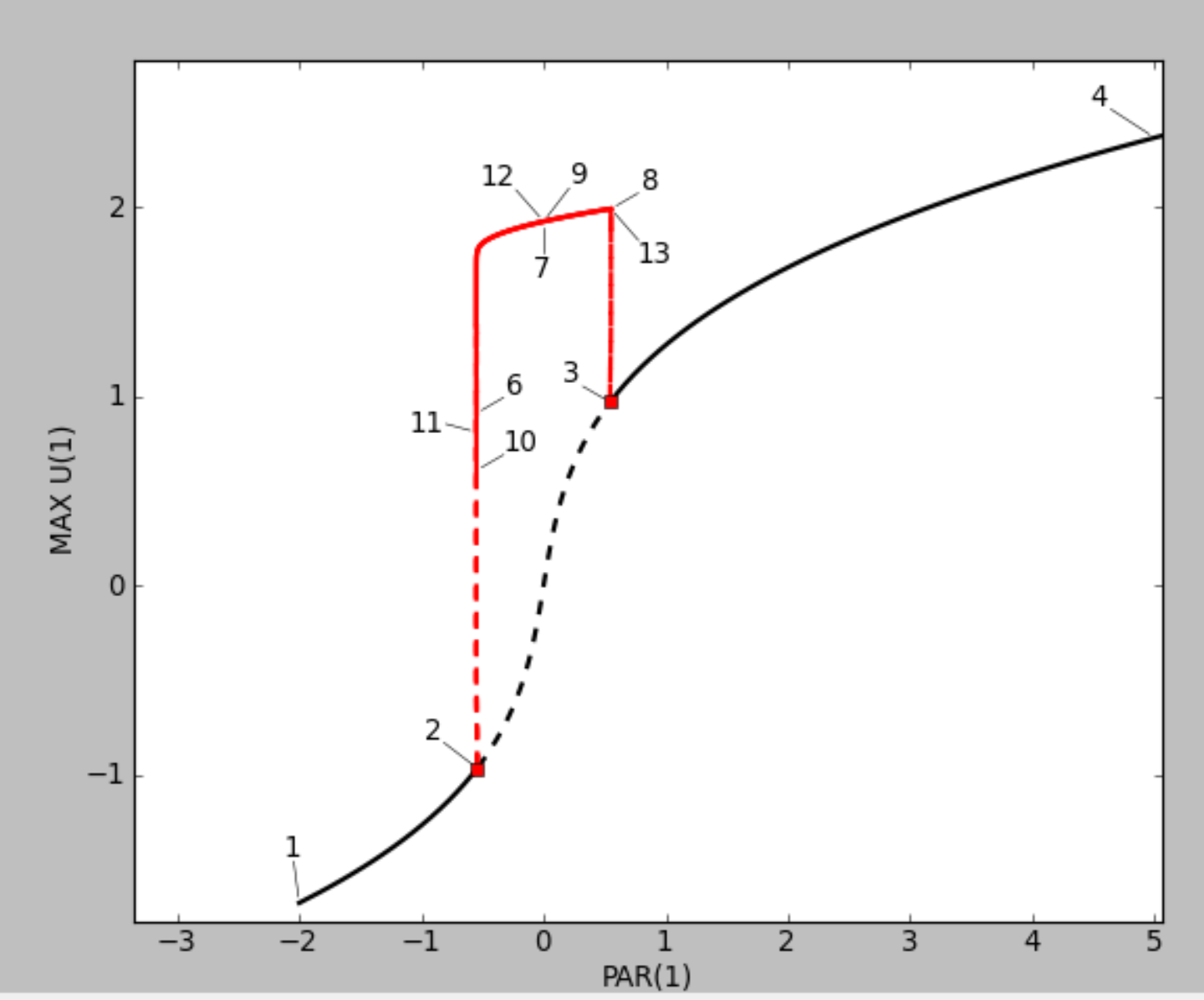
My question is how do I modify the code to get a similar result?
When BifurcationKit is installed, the whole Plots library and GR (whose combination is massive) is installed with it.
Perhaps a more lean approach would be to use the Requries package and add conditional dependencies, so that users don't have to get Plots if they don't want to plot things? For example, have a look of how I have done this in DynamicalBilliards.jl, which extends several PyPlot.jl functions:
https://github.com/JuliaDynamics/DynamicalBilliards.jl/blob/master/src/DynamicalBilliards.jl#L51-L63
Requesting to make these structures mutable so that it would be possible to update hyperparameters during optimisation loops.
parameters = ContinuationPar() # inital hyperparameters

for i=1:10 # some optimisation loop
       parameters.ds *= i*parameters.ds # for example changing ds
end
throws ERROR: setfield! immutable struct of type ContinuationPar cannot be changed
For better visibility and integration of BifurcationKit with SciML, some examples, in particular DAE and PDE, should be formulated using MTK with its automatic Jc features.
Also, BifurcationKit should have better visibility in the SciML ecosystem.
it seems to be ok with ContResult though!
using PseudoArcLengthContinuation, LinearAlgebra, Plots
const PALC = PseudoArcLengthContinuation
using ForwardDiff
using Parameters, Setfield

function f(x, p)
    [p.α*x[1] + x[1]^3 ]
end
function Jf(x, p)
    Jf = zeros(1, 1)
    Jf[1] = p.α+3x[1]^2
    dx -> Jf*dx
end

# eigensolver
struct MyStruct <: PALC.AbstractEigenSolver
end
function (m::MyStruct)(J, nev)
    return [(J(1))[1]], [1.], true, 1
end

Fmit = f
D(f, x, p, dx) = ForwardDiff.derivative(t->f(x .+ t .* dx, p), 0.)
function D(f, x, p, dx)
    ε=1e-10
    (f(x + ε*dx, p) - f(x, p))/ε
end
d1Fmit(x,p,dx1) = D((z, p0) -> Fmit(z, p0), x, p, dx1)
d2Fmit(x,p,dx1,dx2) = D((z, p0) -> d1Fmit(z, p0, dx1), x, p, dx2)
d3Fmit(x,p,dx1,dx2,dx3) = D((z, p0) -> d2Fmit(z, p0, dx1, dx2), x, p, dx3)
jet = (f, d1Fmit, d2Fmit, d3Fmit)
jet = (f, Jf, d2Fmit, d3Fmit)

alpha_min = -10.
alpha_max = 10.
alpha_start = 2.

# options for Newton solver
opt_newton = PALC.NewtonPar(tol = 1e-8, verbose = true, maxIter = 20, eigsolver = MyStruct())
# opt_newton = PALC.NewtonPar(tol = 1e-8, verbose = true, maxIter = 20, eigsolver = MyStruct(), linsolver=GMRESKrylovKit())

# options for continuation
opts_br = ContinuationPar(dsmin = 0.001, dsmax = 0.05, ds = -0.01, pMax = alpha_max, pMin = alpha_min,
	                  detectBifurcation = 2, nev = 30, plotEveryNsteps = 10, newtonOptions = opt_newton,
	                  maxSteps = 100, precisionStability = 1e-6, nInversion = 4, dsminBisection = 1e-7, maxBisectionSteps = 25)

sol_start, _, _ = newton( f, [1.], (α=.1,), opt_newton)
par_mit = (α=alpha_start,)

br, _ = @time PALC.continuation(
    Fmit, Jf,
    sol_start, par_mit, (@lens _.α), opts_br;
    # printSolution = (x, p) -> norm(x),
    # plotSolution = (x, p; kwargs...) -> plotsol!(x ; kwargs...),
    plot = false, verbosity = 3)

br2, _ = continuation(jet..., br, 1, setproperties(opts_br, ds = -0.01, maxSteps = 20), plot = false, printSolution = (x,p) -> x[1], verbosity=3, Jt=Jf)
br3, _ = continuation(jet..., br, 1, setproperties(opts_br, ds = 0.01, maxSteps = 20), plot = false, printSolution = (x,p) -> x[1], verbosity=3, Jt=Jf)

Plots.plot([br,br2,br3])
doesn't work. It does if I uncomment the opt_newton line setting the linear solver. I mention this as a bug because the continuation (without branch switching) seems to work fine, meaning it probably autodetects that the problem is matrix-free but branch switching doesn't?
DiffEqBase is the lowest common denominator for the DiffEq packages, not necessarily the whole SciML ecosystem, and so it has a lot DiffEq dependencies. These are generally not required by downstream packages. If what you're looking for is a way to define problems without having most dependencies, we recommend you use SciMLBase as the dependency since everything like ODEProblem, SteadyStateProblem, etc. is defined there. We basically recommend depending on SciMLBase for problem definitions, and solver packages for specific solvers, but generally most non-SciML packages should not be depending on DiffEqBase directly (given the split of SciMLBase in 2021)
For more details see: https://diffeq.sciml.ai/stable/features/low_dep/ and https://discourse.julialang.org/t/psa-the-right-dependency-to-reduce-from-differentialequations-jl/72757
Let me know if you need any help updating this, though for almost all dependents here it should be a trivial name change as you're actually using pieces from SciMLBase.
Bug report: I was trying to compute a branch of periodic orbits of a forced nonlinear oscillator with shooting when I came across this issue. It happens when the continuation method is used with AbstractShootingProblem and detectBifurcation > 0. The method extractPeriodShooting is called by MonodromyQaD in Floquet.jl, giving the error. Below is a code sample that reproduces the error.
using Revise, Parameters, Setfield, Plots, LinearAlgebra
using DifferentialEquations
using BifurcationKit
const BK = BifurcationKit

# define the sup norm
norminf(x) = norm(x, Inf)

# function to record information from a solution
recordFromSolution(x, p) = (u1 = x[1], u2 = x[2])

####################################################################################################

function F!(f, x, p, t=0)
	@unpack a, b1, b2, d, λ, ω = p
	f[1] = x[2]
	f[2] = - d * x[2] - a * x[1] - b1 * (x[1]^2) - b2 * (x[1]^3) + λ * sin(ω * t)
    return f
end
F(x,p,t) = F!(similar(x),x,p,t)

# Defining the Jacobian
function dF(x,p,t = 0)
	@unpack a, b1, b2, d, λ, ω = p
    M = zeros(2,2)
    M[1,1] = 0
    M[1,2] = 1
    M[2,1] = -a -b1*2*x[1] -b2*3*(x[1]^2)
    M[2,2] = -d
    return M
 end

# parameters of the model
P = @with_kw (a=-1., b1=1., b2=0., d=0.1, λ=0.06, ω=0.81)
par_Helm = P(-1.0, 1.0, 0.0, 0.1, 0.06, 0.81)
par0 = (@set par_Helm.a = -1.15)

# initial condition guess
z0 = [1.; 0.001]
vf = ODEFunction(F; jac = dF)       #ODEfunction with the Jacobian
prob = ODEProblem(vf, z0, (0.0, 1000*2*π/par0.ω), par0)   #ODEProblem encoding
sol = solve(prob, Tsit5())

z0 = sol.u[end]
prob = ODEProblem(vf, z0, (0.0, 2*π/par0.ω), par0)   #ODEProblem encoding
sol = solve(prob, Tsit5())

# this encodes the functional for the Shooting problem
probSh = ShootingProblem(
	# we pass the ODEProblem encoding the flow and the time stepper
	prob, Tsit5(),
	# this is for the phase condition, you can pass your own section as well
	[vec(sol[end])],
	# enable threading
	parallel = true,
	# these are options passed to the ODE time stepper
	atol = 1e-10, rtol = 1e-8)

# Newton interation for low energy level
zp0 = vcat(vec(sol[end]),2*π/par_Helm.ω)

ls = GMRESIterativeSolvers(reltol = 1e-7, N = length(zp0), maxiter = 100)
newtonOpt = NewtonPar(verbose = true, tol = 1e-8, maxIter = 25, linsolver = ls)

# continuation options
opts_cont = ContinuationPar(dsmin = 0.001, dsmax = 1.0, ds= 0.01, pMin = 0.02, pMax = 0.1,
	maxSteps = 50, newtonOptions = newtonOpt, nev = 2,
	# options to detect bifurcations
	detectBifurcation = 3,   # this gives an error!
        detectFold = true, nInversion = 8, maxBisectionSteps = 25,
	precisionStability = 1e-8, saveSolEveryStep = 1)

br, = continuation(
    probSh,
    zp0,
    par0,
    (@lens _.λ),
    opts_cont,
    linearAlgo = MatrixFreeBLS(@set ls.N = ls.N + 1);
    verbosity = 3,
    plot = true,
    recordFromSolution = recordFromSolution,
	normC = norminf
)Hi Romain,
Let me preface this by saying a huge thank you for your invaluable work on this package. At some point this year I am hoping to release my own amateurish package about numerical continuation methods in atomistic simulation of materials and it will be based around BifurcationKit.jl. I have also cited the paper about this package in a recent preprint.
Onto to the issue - title says it all really. It looks to me like any adjustement in dotPALC is not reflected in the computation of the predictor with BorderedPred(), which in my case leads to the breakdown of the continuation routine.
If in my continuation routine I use theta = 0.5 and
tangentAlgo = BorderedPred(), dotPALC = (x, y) -> dot(x, y)/length(x)
then everything runs well, but to achieve the desired step size control, I need to pass something dsmin = 0.00001, dsmax = 0.001, ds= 0.0004 (which would have to be decreased even further as if I was to increase the size of my computational domain - the number of atoms I simulate).
As noted in the documentation, I would like to instead pass
tangentAlgo = BorderedPred(), dotPALC = (x, y) -> dot(x, y)
but when I do that and run the routine, I get an error PosDefException: matrix is not positive definite; Cholesky factorization failed. If on the other hand I pass
tangentAlgo = SecantPred(), dotPALC = (x, y) -> dot(x, y)
then everything is well again and this time dsmin, dsmax, ds have to be adjusted to more reasonable values, which crucially are (more or less) domain-size independent.
I would really like to use BorderedPred() though and having browsed the source code, it looks like this might have something to do with the function `DotTheta()' in Predictor.jl. I think this should be easily fixable or perhaps I am simply misunderstanding something, but I thought I would draw your attention to it just in case. Thanks!
I just got an upgrade conficlt because of an old version of JLD2 and I thought "Where does it come from?" because I've never installed JLD2. Turns out it was coming from here.
It made me wonder, why would such a front-end package be a dependency here?
First, sorry for all the troubles!
I have been trying to create some very simple bifurcation diagrams using deflated continuations; however, I have not been able to get it to work. I think I simply do not understand how to give some of the input properly.
The first example is a very simple system:
dX/dt = p -d*X (p and d are parameters)
I create the system using Catalyst.
For reference, I have been using the deflated continuation example at https://rveltz.github.io/BifurcationKit.jl/dev/DeflatedContinuation/, as well as the @reaction_network example discussion at #27.
In my first try, I simply take the example in the docs, but swaps stuff out for what I got in my system:
# Fetch packages.
using Catalyst
using BifurcationKit, LinearAlgebra, Setfield, SparseArrays, Plots

# Create functions.
rn = @reaction_network begin
    p, 0 --> X
    d, X --> 0
end p d;
odefun = ODEFunction(convert(ODESystem,rn),jac=true)
F = (u,p) -> odefun(u,p,0)
J = (u,p) -> odefun.jac(u,p,0);

# Set initial parameter values.
p = (p=1.,d=0.1);
# Sets initial guess
x0 = 0.5;

# Set solving options
opts = BifurcationKit.ContinuationPar(dsmax = 0.051, dsmin = 1e-3, ds=0.001, maxSteps = 140, pMin = -3., saveSolEveryStep = 0, newtonOptions = NewtonPar(tol = 1e-8, verbose = false), saveEigenvectors = false);

# Set Deflation Options
DO = DeflationOperator(2.0, dot, .001, [[0.]]);

# Create bifurcation diagram
brdc, = continuation(F,J, x0, (@lens _),opts,DO; showplot=false, verbosity = 0);

# Plot the diagram
plot(brdc[1])
This code runs without error, but the output is weird, and rightly so, since the algorithm doesn't have the adequate information. It is when I move on from this I start to be confussed. First, I have a question regarding the creation of the DeflationOperator though:
dot?). Finally, the fourth argument is an array with roots which I want to avoid? Exactly how should I give it here? Is it roots which I want to ignore, or is it to help the algorithm to find all the roots at the starting condition, but do I then need to give all of the roots except for one (with the algorithm finding the last one)? In the doc example, a root at 0 is given, but the algorithm finds and uses 2 more. If I don't want to skip any roots, can I give this one as an empty array?Next, I try to give the systems parameter values as an input as well, I try a few different ones, the only one that succeeds is:
brdc, = continuation(F,J,p, (@lens _.p),opts,DO; showplot=false, verbosity = 0);x0? Other alternatives such as:brdc, = continuation(F,J,x0, p, (@lens _.p),opts,DO; showplot=false, verbosity = 0);
brdc, = continuation(F,J,p, x0, (@lens _.p),opts,DO; showplot=false, verbosity = 0);fails
Next, I try a slightly more complicated system:
# Fetch packages.
using Catalyst
using BifurcationKit, LinearAlgebra, Setfield, SparseArrays, Plots

# Create functions.
rn2 = @reaction_network begin
    (v0+(S*X)^n/((S*X)^n+(D*A)^n+1),1), ∅ ↔ X
    (τ*X,τ), ∅ ↔ A
end v0 S n D τ;
odefun2 = ODEFunction(convert(ODESystem,rn2),jac=true)
F2 = (u,p) -> odefun2(u,p,0)
J2 = (u,p) -> odefun2.jac(u,p,0);

# Set initial parameter values.
p2 = (v0=0.1, S=1., n=3, D=2., τ=0.01);
# Sets initial guess
x02 = [0.5, 0.5];

# Set solving options
opts2 = BifurcationKit.ContinuationPar(dsmax = 0.051, dsmin = 1e-3, ds=0.001, maxSteps = 1000000, pMin = 0.1, pMax = 5., saveSolEveryStep = 0, newtonOptions = NewtonPar(tol = 1e-8, verbose = false), saveEigenvectors = false);

# Set Deflation Options
DO2 = DeflationOperator(2.0, dot, .001, [[0.,0.]]);

# Create bifurcation diagram
brdc2, = continuation(F2,J2,p2, (@lens _.S),opts2,DO2; showplot=false, verbosity = 0);

# Plot the diagram
plot(brdc2[1])
This does give me parts of the diagram as output, but not everything (it is one of those bistable switches, but I only get the first third, up until it is supposed to turn over and go backwards):

I have tried modifying option values, as well as adding
termination_condition(x, f, J, residual, iteration, niter, options; kwargs...) = residual <1e3
root_search(x,p,id) = x .+ rand(length(x))
but didn't get it to work. What is going wrong here, and what should I do to modify?
Hello,
I try to compute a bifurcation diagram using the bifurcationdiagram function. The system is a 2 variable ODE originating from a biochemical reaction network. This is the example:
# Fetch packages.
using BifurcationKit
using Catalyst
using OrdinaryDiffEq
using Plots
using Setfield

# Declare our model.
hillAR(x1,x2,v,K,n) = (v*x1^n)/(x1^n+x2^n+K^n)
ss_network = @reaction_network begin
    v0+hillAR(S*X,D*Y,v,K,n), ∅ → X
    v0+hillAR(S*Y,D*X,v,K,n), ∅ → Y
    1,(X,Y) → ∅
end S D v0 v n K;

# Generate system functions.
odefun = ODEFunction(convert(ODESystem,rn),jac=true)
F = (u,p) -> odefun(u,p,0)
J = (u,p) -> odefun.jac(u,p,0);
jet = BifurcationKit.getJet(F, J; matrixfree=false)

# Select parameters
params_in = [1.0,0.5,0.1,1.0,2,0.5];
p_idx = 1;
p_span = (0.1,2.5)
params = setindex!(copy(params_in),p_span[1],p_idx);

# Set options.
dsmax = params[p_idx]/500
dsmin = min(params[p_idx]/10000,1e-4)
ds = sqrt(dsmax*dsmin);
opts_br = ContinuationPar(pMin = p_span[1], pMax = p_span[2], dsmax = dsmax, dsmin = dsmin, ds=ds, maxSteps = 1000000,
    detectBifurcation = 3,
    nInversion = 6, maxBisectionSteps = 25,
    nev = 3);

# Compute diagram.
bif = bifurcationdiagram(jet..., u0, params, (@lens _[p_idx]), 3,
    (x,p,level)->setproperties(opts_br);
    tangentAlgo = NaturalPred(),
    recordFromSolution=(x, p) -> x[v_idx], verbosity = 0, plot=false);

# Plot the diagram.
plot(bif)
Now, this produces the print:
##################################################
---> Automatic computation of bifurcation diagram

────────────────────────────────────────────────────────────────────────────────
--> New branch, level = 2, dim(Kernel) = 1, code = 0, from bp #1 at p = 0.858837922561846, type = bp
- #  1,    bp at p ≈ +0.85883792 ∈ (+0.85883753, +0.85883792), |δp|=4e-07, [converged], δ = ( 1,  0), step = 3797, eigenelements in eig[3798], ind_ev =   1
----> From Pitchfork
- #  1,    bp at p ≈ +0.85883792 ∈ (+0.85883753, +0.85883792), |δp|=4e-07, [converged], δ = ( 1,  0), step = 3797, eigenelements in eig[3798], ind_ev =   1
────────────────────────────────────────────────────────────────────────────────
--> New branch, level = 2, dim(Kernel) = 1, code = 0, from bp #2 at p = 1.0061644362337048, type = bp
- #  2,    bp at p ≈ +1.00616444 ∈ (+1.00616439, +1.00616444), |δp|=5e-08, [converged], δ = (-1,  0), step = 4534, eigenelements in eig[4535], ind_ev =   1
----> From Pitchfork
- #  2,    bp at p ≈ +1.00616444 ∈ (+1.00616439, +1.00616444), |δp|=5e-08, [converged], δ = (-1,  0), step = 4534, eigenelements in eig[4535], ind_ev =   1
and the plot:

However, the bifurcation diagram should look more like this:

Basically, in the two branch (pitchfork?) points, two branches go out, which (via two fold points) later connect to the other pitchfork bifurcation.
The code above generates a single branch, with 4 children, if I plot each
plot(plot(bif.γ),plot(bif.child[1].γ),plot(bif.child[2].γ),plot(bif.child[3].γ),plot(bif.child[4].γ),size=(1200,600))I get

this makes it seem like the solver detects that there are two branches going out from each pitchfork point. However, when it tracks these two, it simply follows the original path back/forward towards the end, creating some overlap.
I have tried changing options in (x,p,level)->setproperties(opts_br), using various combinations of what is used in the first example at https://bifurcationkit.github.io/BifurcationKitDocs.jl/dev/BifurcationDiagram/, however, with no luck. I also tried removing tangentAlgo = NaturalPred(), but for large level Julia crashes, and for smaller when I try to print the bifurcation diagram I get no output.
I have also tried making the sign of ds iterate with the level, using
(x,p,level)->setproperties(opts_br;ds=-ds*(-1)^level)but it didn't work.
Is it just that I am missing some option to make it properly detect the branches, or is there some other problem?
Hi there,
I'm trying to come up with a simple example for the bifurcation of 1-dimensional system to contribute to the documentation, under guidance of @gszep . I have the example running, by altering the code https://rveltz.github.io/BifurcationKit.jl/dev/iterator/# , but there are some things that are not yet clear enough for me.
What I really want to know is what is the allowed return types for both the vector field f and the Jacobian. The code has:
Jac_m = (x, p) -> diagm(0 => 1.0 .- x.^k)
but it was confusing for me because when I tried other types of Jac_m I got errors (I am not reporting errors here until I first see what is the expected form of Jacobian). I also tried to use the output of ForwardDiff.jacobian, also getting errors.
So, can you please document somewhere centrally in the documentation what is the expected forms for f, J? Not only what are the input arguments, but what is the expected output. The documentation of e.g. https://rveltz.github.io/BifurcationKit.jl/dev/library/#BifurcationKit.continuation does not discuss with clarity what J should be. There you can also provide tips and tricks, as e.g. the above usage of diagm is definitely something advanced for me, I would expected a 1-element matrix as return type in this example.
A comment on how the docstring is structured: it provides:
F = (x, p) -> F(x, p)This, almost always, is invalid Julia code. If F is an existing function, here you are redefining it as an anonymous function F, and Julia will just error. It also doesn't highlight what is the return type of F, yet repeats what are the expected input arguments.
Why not consider replacing it with the more valid F(x,p)::AbstractVector, or simply explicitly write things out as e.g. "F is a function with input arguments (x, p) returning a vector r that represents the vector field of the dynamics".
Are static vectors supported?
I'm trying to save the continuation results by setting the keyword argument saveToFile=true, however it doesn't seen to work. I'm just playing with the temperature model in the tutorial:
using BifurcationKit, LinearAlgebra, Plots, Parameters, Setfield
# Setfield.jl is used to provide the parameter axis @lens
const BK = BifurcationKit

N(x; a = 0.5, b = 0.01) = 1 + (x + a*x^2)/(1 + b*x^2)

function F_chan(x, p)
    @unpack α, β = p
    f = similar(x)
    n = length(x)
    f[1] = x[1] - β
    f[n] = x[n] - β
    for i=2:n-1
        f[i] = (x[i-1] - 2 * x[i] + x[i+1]) * (n-1)^2 + α * N(x[i], b = β)
    end
    return f
end

n = 101
sol = [(i-1)*(n-i)/n^2+0.1 for i=1:n]

# set of parameters
par = (α = 3.3, β = 0.01)

optnewton = NewtonPar(tol = 1e-11, verbose = false)

out, = @time newton( F_chan, sol, par, optnewton)

optcont = ContinuationPar(dsmin = 0.01, dsmax = 0.2, ds= 0.1, pMin = 0., pMax = 4.1, saveToFile=true,
    newtonOptions = NewtonPar(maxIter = 10, tol = 1e-9))

br, = continuation(F_chan, out, par, (@lens _.α),
        optcont; plot = false, verbosity = 1)
but I get the following error:
  0.236941 seconds (846.97 k allocations: 45.750 MiB, 98.13% compilation time)
UndefVarError: saveToFile not defined

Stacktrace:
 [1] continuation!(it::ContIterable{typeof(F_chan), BifurcationKit.var"#148#150"{typeof(F_chan)}, Vector{Float64}, NamedTuple{(:α, :β), Tuple{Float64, Float64}}, Setfield.PropertyLens{:α}, Float64, DefaultLS, DefaultEig{typeof(real)}, SecantPred, MatrixBLS{Nothing}, BifurcationKit.var"#126#134"{BifurcationKit.var"#126#127#135"}, BifurcationKit.var"#128#136"{BifurcationKit.var"#128#129#137"}, typeof(norm), BifurcationKit.DotTheta{BifurcationKit.var"#169#171", BifurcationKit.var"#170#172"}, typeof(BifurcationKit.finaliseDefault), typeof(BifurcationKit.cbDefault), Nothing, String}, state::ContState{BorderedArray{Vector{Float64}, Float64}, Float64, Nothing, Nothing, Tuple{Nothing, Nothing}}, contRes::ContResult{NamedTuple{(:x, :param, :itnewton, :itlinear, :ds, :θ, :n_unstable, :n_imag, :stable, :step), Tuple{Float64, Float64, Int64, Int64, Float64, Float64, Int64, Int64, Nothing, Int64}}, Nothing, Nothing, BifurcationKit.SpecialPoint{Float64, NamedTuple{(:x,), Tuple{Float64}}, Vector{Float64}}, Nothing, ContinuationPar{Float64, DefaultLS, DefaultEig{typeof(real)}}, Nothing, NamedTuple{(:α, :β), Tuple{Float64, Float64}}, Setfield.PropertyLens{:α}})
   @ BifurcationKit C:\Users\yhcha\.julia\packages\BifurcationKit\eoTLY\src\Continuation.jl:446
 [2] continuation(it::ContIterable{typeof(F_chan), BifurcationKit.var"#148#150"{typeof(F_chan)}, Vector{Float64}, NamedTuple{(:α, :β), Tuple{Float64, Float64}}, Setfield.PropertyLens{:α}, Float64, DefaultLS, DefaultEig{typeof(real)}, SecantPred, MatrixBLS{Nothing}, BifurcationKit.var"#126#134"{BifurcationKit.var"#126#127#135"}, BifurcationKit.var"#128#136"{BifurcationKit.var"#128#129#137"}, typeof(norm), BifurcationKit.DotTheta{BifurcationKit.var"#169#171", BifurcationKit.var"#170#172"}, typeof(BifurcationKit.finaliseDefault), typeof(BifurcationKit.cbDefault), Nothing, String})
   @ BifurcationKit C:\Users\yhcha\.julia\packages\BifurcationKit\eoTLY\src\Continuation.jl:485
 [3] continuation(Fhandle::Function, Jhandle::Function, x0::Vector{Float64}, par::NamedTuple{(:α, :β), Tuple{Float64, Float64}}, lens::Setfield.PropertyLens{:α}, contParams::ContinuationPar{Float64, DefaultLS, DefaultEig{typeof(real)}}, linearAlgo::MatrixBLS{Nothing}; bothside::Bool, kwargs::Base.Pairs{Symbol, Integer, Tuple{Symbol, Symbol}, NamedTuple{(:plot, :verbosity), Tuple{Bool, Int64}}})
   @ BifurcationKit C:\Users\yhcha\.julia\packages\BifurcationKit\eoTLY\src\Continuation.jl:0
 [4] #continuation#146
   @ C:\Users\yhcha\.julia\packages\BifurcationKit\eoTLY\src\Continuation.jl:567 [inlined]
 [5] #continuation#147
   @ C:\Users\yhcha\.julia\packages\BifurcationKit\eoTLY\src\Continuation.jl:570 [inlined]
 [6] top-level scope
   @ In[153]:32
 [7] eval
   @ .\boot.jl:373 [inlined]
 [8] include_string(mapexpr::typeof(REPL.softscope), mod::Module, code::String, filename::String)
   @ Base .\loading.jl:1196
I am running the tutorial, trying to figure out how to plot periodic orbits in ODE bifurcation diagrams.
I am trying the tutorial in: https://rveltz.github.io/BifurcationKit.jl/dev/tutorials/ode/tutorialsODE/#Neural-mass-equation-(Hopf-aBS) however, the section on "Branch of periodic orbits with Trapezoid method" gives an error:
UndefVarError: getTrajectory not defined

Stacktrace:
  [1] (::var"#5#8")(x::Vector{Float64}, p::NamedTuple{(:prob, :p), Tuple{PeriodicOrbitTrapProblem{typeof(TMvf), typeof(dTMvf), Nothing, Nothing, Nothing, Vector{Float64}, DefaultLS, BifurcationKit.TimeMesh{Int64}, Nothing}, Float64}})
    @ Main ./In[5]:7
  [2] #808#809
    @ ~/.julia/packages/BifurcationKit/eoTLY/src/periodicorbit/PeriodicOrbitUtils.jl:81 [inlined]
  [3] #808
    @ ~/.julia/packages/BifurcationKit/eoTLY/src/periodicorbit/PeriodicOrbitUtils.jl:81 [inlined]
  [4] ContResult(it::ContIterable{PeriodicOrbitTrapProblem{typeof(TMvf), typeof(dTMvf), Nothing, Nothing, Nothing, Vector{Float64}, DefaultLS, BifurcationKit.TimeMesh{Int64}, Nothing}, BifurcationKit.var"#753#758"{PeriodicOrbitTrapProblem{typeof(TMvf), typeof(dTMvf), Nothing, Nothing, Nothing, Vector{Float64}, DefaultLS, BifurcationKit.TimeMesh{Int64}, Nothing}}, Vector{Float64}, NamedTuple{(:α, :τ, :J, :E0, :τD, :U0, :τF, :τS), NTuple{8, Float64}}, Setfield.PropertyLens{:E0}, Float64, BifurcationKit.FloquetWrapperLS{DefaultLS}, FloquetQaD{DefaultEig{typeof(abs)}}, SecantPred, BorderingBLS{BifurcationKit.FloquetWrapperLS{DefaultLS}, Float64}, BifurcationKit.var"#818#822"{BifurcationKit.var"#818#819#823"{PeriodicOrbitTrapProblem{typeof(TMvf), typeof(dTMvf), Nothing, Nothing, Nothing, Vector{Float64}, DefaultLS, BifurcationKit.TimeMesh{Int64}, Nothing}, var"#6#9"}}, BifurcationKit.var"#808#812"{BifurcationKit.var"#808#809#813"{PeriodicOrbitTrapProblem{typeof(TMvf), typeof(dTMvf), Nothing, Nothing, Nothing, Vector{Float64}, DefaultLS, BifurcationKit.TimeMesh{Int64}, Nothing}, var"#5#8"}}, typeof(norminf), BifurcationKit.DotTheta{BifurcationKit.var"#169#171", BifurcationKit.var"#170#172"}, BifurcationKit.var"#800#804"{BifurcationKit.var"#800#801#805"{PeriodicOrbitTrapProblem{typeof(TMvf), typeof(dTMvf), Nothing, Nothing, Nothing, Vector{Float64}, DefaultLS, BifurcationKit.TimeMesh{Int64}, Nothing}, Int64}}, typeof(BifurcationKit.cbDefault), Nothing, String}, state::ContState{BorderedArray{Vector{Float64}, Float64}, Float64, Vector{ComplexF64}, Matrix{ComplexF64}, Tuple{Nothing, Nothing}})
    @ BifurcationKit ~/.julia/packages/BifurcationKit/eoTLY/src/Continuation.jl:238
  [5] continuation(it::ContIterable{PeriodicOrbitTrapProblem{typeof(TMvf), typeof(dTMvf), Nothing, Nothing, Nothing, Vector{Float64}, DefaultLS, BifurcationKit.TimeMesh{Int64}, Nothing}, BifurcationKit.var"#753#758"{PeriodicOrbitTrapProblem{typeof(TMvf), typeof(dTMvf), Nothing, Nothing, Nothing, Vector{Float64}, DefaultLS, BifurcationKit.TimeMesh{Int64}, Nothing}}, Vector{Float64}, NamedTuple{(:α, :τ, :J, :E0, :τD, :U0, :τF, :τS), NTuple{8, Float64}}, Setfield.PropertyLens{:E0}, Float64, BifurcationKit.FloquetWrapperLS{DefaultLS}, FloquetQaD{DefaultEig{typeof(abs)}}, SecantPred, BorderingBLS{BifurcationKit.FloquetWrapperLS{DefaultLS}, Float64}, BifurcationKit.var"#818#822"{BifurcationKit.var"#818#819#823"{PeriodicOrbitTrapProblem{typeof(TMvf), typeof(dTMvf), Nothing, Nothing, Nothing, Vector{Float64}, DefaultLS, BifurcationKit.TimeMesh{Int64}, Nothing}, var"#6#9"}}, BifurcationKit.var"#808#812"{BifurcationKit.var"#808#809#813"{PeriodicOrbitTrapProblem{typeof(TMvf), typeof(dTMvf), Nothing, Nothing, Nothing, Vector{Float64}, DefaultLS, BifurcationKit.TimeMesh{Int64}, Nothing}, var"#5#8"}}, typeof(norminf), BifurcationKit.DotTheta{BifurcationKit.var"#169#171", BifurcationKit.var"#170#172"}, BifurcationKit.var"#800#804"{BifurcationKit.var"#800#801#805"{PeriodicOrbitTrapProblem{typeof(TMvf), typeof(dTMvf), Nothing, Nothing, Nothing, Vector{Float64}, DefaultLS, BifurcationKit.TimeMesh{Int64}, Nothing}, Int64}}, typeof(BifurcationKit.cbDefault), Nothing, String})
    @ BifurcationKit ~/.julia/packages/BifurcationKit/eoTLY/src/Continuation.jl:482
  [6] continuation(Fhandle::PeriodicOrbitTrapProblem{typeof(TMvf), typeof(dTMvf), Nothing, Nothing, Nothing, Vector{Float64}, DefaultLS, BifurcationKit.TimeMesh{Int64}, Nothing}, Jhandle::Function, x0::Vector{Float64}, par::NamedTuple{(:α, :τ, :J, :E0, :τD, :U0, :τF, :τS), NTuple{8, Float64}}, lens::Setfield.PropertyLens{:E0}, contParams::ContinuationPar{Float64, BifurcationKit.FloquetWrapperLS{DefaultLS}, FloquetQaD{DefaultEig{typeof(abs)}}}, linearAlgo::BorderingBLS{BifurcationKit.FloquetWrapperLS{DefaultLS}, Float64}; bothside::Bool, kwargs::Base.Pairs{Symbol, Any, NTuple{7, Symbol}, NamedTuple{(:recordFromSolution, :linearPO, :verbosity, :plot, :plotSolution, :normC, :finaliseSolution), Tuple{BifurcationKit.var"#808#812"{BifurcationKit.var"#808#809#813"{PeriodicOrbitTrapProblem{typeof(TMvf), typeof(dTMvf), Nothing, Nothing, Nothing, Vector{Float64}, DefaultLS, BifurcationKit.TimeMesh{Int64}, Nothing}, var"#5#8"}}, Symbol, Int64, Bool, BifurcationKit.var"#818#822"{BifurcationKit.var"#818#819#823"{PeriodicOrbitTrapProblem{typeof(TMvf), typeof(dTMvf), Nothing, Nothing, Nothing, Vector{Float64}, DefaultLS, BifurcationKit.TimeMesh{Int64}, Nothing}, var"#6#9"}}, typeof(norminf), BifurcationKit.var"#800#804"{BifurcationKit.var"#800#801#805"{PeriodicOrbitTrapProblem{typeof(TMvf), typeof(dTMvf), Nothing, Nothing, Nothing, Vector{Float64}, DefaultLS, BifurcationKit.TimeMesh{Int64}, Nothing}, Int64}}}}})
    @ BifurcationKit ~/.julia/packages/BifurcationKit/eoTLY/src/Continuation.jl:0
  [7] continuationPOTrap(prob::PeriodicOrbitTrapProblem{typeof(TMvf), typeof(dTMvf), Nothing, Nothing, Nothing, Vector{Float64}, DefaultLS, BifurcationKit.TimeMesh{Int64}, Nothing}, orbitguess::Vector{Float64}, par::NamedTuple{(:α, :τ, :J, :E0, :τD, :U0, :τF, :τS), NTuple{8, Float64}}, lens::Setfield.PropertyLens{:E0}, contParams::ContinuationPar{Float64, DefaultLS, DefaultEig{typeof(real)}}, linearAlgo::BorderingBLS{DefaultLS, Float64}; jacobianPO::Symbol, updateSectionEveryStep::Int64, kwargs::Base.Pairs{Symbol, Any, NTuple{6, Symbol}, NamedTuple{(:recordFromSolution, :linearPO, :verbosity, :plot, :plotSolution, :normC), Tuple{var"#5#8", Symbol, Int64, Bool, var"#6#9", typeof(norminf)}}})
    @ BifurcationKit ~/.julia/packages/BifurcationKit/eoTLY/src/periodicorbit/PeriodicOrbitTrapeze.jl:916
  [8] #continuation#763
    @ ~/.julia/packages/BifurcationKit/eoTLY/src/periodicorbit/PeriodicOrbitTrapeze.jl:978 [inlined]
  [9] continuation(F::typeof(TMvf), dF::typeof(dTMvf), d2F::BifurcationKit.var"#d2f#284"{BifurcationKit.var"#d1f#282"{typeof(TMvf)}}, d3F::BifurcationKit.var"#d3f#286"{BifurcationKit.var"#d2f#284"{BifurcationKit.var"#d1f#282"{typeof(TMvf)}}}, br::ContResult{NamedTuple{(:E, :x, :u, :param, :itnewton, :itlinear, :ds, :θ, :n_unstable, :n_imag, :stable, :step), Tuple{Float64, Float64, Float64, Float64, Int64, Int64, Float64, Float64, Int64, Int64, Bool, Int64}}, Vector{ComplexF64}, Matrix{ComplexF64}, BifurcationKit.SpecialPoint{Float64, NamedTuple{(:E, :x, :u), Tuple{Float64, Float64, Float64}}, Vector{Float64}}, Nothing, ContinuationPar{Float64, DefaultLS, DefaultEig{typeof(real)}}, Nothing, NamedTuple{(:α, :τ, :J, :E0, :τD, :U0, :τF, :τS), NTuple{8, Float64}}, Setfield.PropertyLens{:E0}}, ind_bif::Int64, _contParams::ContinuationPar{Float64, DefaultLS, DefaultEig{typeof(real)}}, prob::PeriodicOrbitTrapProblem{Nothing, Nothing, Nothing, Nothing, Nothing, Nothing, DefaultLS, BifurcationKit.TimeMesh{Int64}, Nothing}; Jᵗ::Nothing, δ::Float64, δp::Nothing, ampfactor::Int64, usedeflation::Bool, nev::Int64, updateSectionEveryStep::Int64, kwargs::Base.Pairs{Symbol, Any, NTuple{6, Symbol}, NamedTuple{(:linearPO, :verbosity, :plot, :recordFromSolution, :plotSolution, :normC), Tuple{Symbol, Int64, Bool, var"#5#8", var"#6#9", typeof(norminf)}}})
    @ BifurcationKit ~/.julia/packages/BifurcationKit/eoTLY/src/periodicorbit/PeriodicOrbits.jl:410
 [10] top-level scope
    @ In[5]:21
 [11] eval
    @ ./boot.jl:373 [inlined]
 [12] include_string(mapexpr::typeof(REPL.softscope), mod::Module, code::String, filename::String)
    @ Base ./loading.jl:1196
I get this after copying (and running) all the code in the tutorial
using Revise, ForwardDiff, Parameters, Setfield, Plots, LinearAlgebra
using BifurcationKit
const BK = BifurcationKit

# sup norm
norminf(x) = norm(x, Inf)

# vector field
function TMvf!(dz, z, p, t)
	@unpack J, α, E0, τ, τD, τF, U0 = p
	E, x, u = z
	SS0 = J * u * x * E + E0
	SS1 = α * log(1 + exp(SS0 / α))
	dz[1] = (-E + SS1) / τ
	dz[2] =	(1.0 - x) / τD - u * x * E
	dz[3] = (U0 - u) / τF +  U0 * (1.0 - u) * E
	dz
end

# out of place method
TMvf(z, p) = TMvf!(similar(z), z, p, 0)

# we group the differentials together
dTMvf(z,p) = ForwardDiff.jacobian(x -> TMvf(x,p), z)
jet = BK.getJet(TMvf, dTMvf)

# parameter values
par_tm = (α = 1.5, τ = 0.013, J = 3.07, E0 = -2.0, τD = 0.200, U0 = 0.3, τF = 1.5, τS = 0.007)

# initial condition
z0 = [0.238616, 0.982747, 0.367876]

# continuation options
opts_br = ContinuationPar(pMin = -10.0, pMax = -0.9,
	# parameters to have a smooth result
	ds = 0.04, dsmax = 0.05,
	# this is to detect bifurcation points precisely with bisection
	detectBifurcation = 3,
	# Optional: bisection options for locating bifurcations
	nInversion = 8, maxBisectionSteps = 25, nev = 3)

# continuation of equilibria
br, = continuation(TMvf, dTMvf, z0, par_tm, (@lens _.E0), opts_br;
	recordFromSolution = (x, p) -> (E = x[1], x = x[2], u = x[3]),
	tangentAlgo = BorderedPred(),
	plot = true, normC = norminf)

scene = plot(br, plotfold=false, markersize=3, legend=:topleft)

br

# newton parameters
optn_po = NewtonPar(verbose = true, tol = 1e-8,  maxIter = 10)

# continuation parameters
opts_po_cont = ContinuationPar(dsmax = 0.1, ds= -0.0001, dsmin = 1e-4, pMax = 0., pMin=-5.,
	maxSteps = 110, newtonOptions = (@set optn_po.tol = 1e-7),
	nev = 3, precisionStability = 1e-8, detectBifurcation = 3, plotEveryStep = 10, saveSolEveryStep=1)

# arguments for periodic orbits
args_po = (	recordFromSolution = (x, p) -> (xtt = BK.getTrajectory(p.prob, x, p.p);
		return (max = maximum(xtt.u[1,:]),
				min = minimum(xtt.u[1,:]),
				period = x[end])),
	plotSolution = (x, p; k...) -> begin
		xtt = BK.getTrajectory(p.prob, x, p.p)
		plot!(xtt.t, xtt.u[1,:]; label = "E", k...)
		plot!(xtt.t, xtt.u[2,:]; label = "x", k...)
		plot!(xtt.t, xtt.u[3,:]; label = "u", k...)
		plot!(br,subplot=1, putbifptlegend = false)
		end,
	normC = norminf)

Mt = 200 # number of time sections
	br_potrap, utrap = continuation(jet...,
	# we want to branch form the 4th bif. point
	br, 4, opts_po_cont,
	# we want to use the Trapeze method to locate PO
	PeriodicOrbitTrapProblem(M = Mt);
	# this jacobian is specific to ODEs
	# it is computed using AD and
	# updated inplace
	linearPO = :Dense,
	# regular continuation options
	verbosity = 2,	plot = true,
	args_po...)

scene = plot(br, br_potrap, markersize = 3)
plot!(scene, br_potrap.param, br_potrap.min, label = "")
Indeed, just trying to access the getTrajectory function:
BK.getTrajectorygives the error. I checked, and I have the latest version of BifurcationKit ( [0f109fa4] BifurcationKit v0.1.11).
Hi, I am thinking about using your package. My first try would be to join this with my package VoronoiFVM.jl.
I understand that for the problem call back one can either pass F(x,p) or F(x,p) and J(x,p) together.
As in my code I am calculating F and (sparse) J at the same time using ForwardDiff and DiffResults I wonder if it
would be possible to have another option which allows to pass something like F_and_J(x,p) ?
it would be useful to be able to record vectors of solutions during continuation method. Suppose I am interested in recording the first and third component of my ode system then I would call
Cont.continuation( .... recordfunction = u -> [ u[1], u[3] ] )If u contained a spatial system then a more interesting recordfunction call could be to segment out a pattern and record some statistics on that pattern.. a fourier transform perhaps?
this should not interfere with printsolution or plotBranch
A quick thing. Doesn't matter much but realised that it seemed like this was missing, so figured I'd add it here.
Various methods have an option verbosity, which can carry between 0 and 3 (or 5). However, nowhere does it seem to say exactly what these various levels actually do. testing various things mostly solves it, but could possibly be useful to add in the docs some day (although not of high priority).
This is affecting BifurcationInference.jl is there a new default setting I am not aware of?
Feature request: use Brent's method for bifurcation location. Should be as robust and faster than bisection. There's a julia implementation over at Roots.jl (although the algorithm as described on wikipedia might be sufficient if you don't want to depend on Roots)
I may be misunderstanding something, but it seems that the continuation function is saving incorrect equilibrium values to the ContResult object. In particular, I was looking at the following example.
using ForwardDiff, Parameters, Setfield, Plots, LinearAlgebra, SparseArrays
using BifurcationKit
const BK = BifurcationKit

F(x,p) = @. (x^2 - p)
JacF(x,p) = spdiagm(0=> 2. .* x)

opts = ContinuationPar(detectBifurcation = 3, dsmax = 0.1, dsmin = 1e-3, ds = -0.001, maxSteps = 130, pMin = -3., pMax = 1., saveSolEveryStep = 0, newtonOptions = NewtonPar(tol = 1e-8, verbose = true));

iter = BK.ContIterable(F, JacF, [-0.9], 1., (@lens _), opts; verbosity = 2);
If I run continuation!(iter), the resulting branch covers the positive equilibria (sqrt(p)) twice and misses the negative equilibria (-sqrt(p)) (despite passing a negative initial condition). In contrast, if I iterate the ContInterable by hand, then PALC correctly identifies both positive and negative equilibria.
res = ContResult(iter, iterate(iter)[1])
resx = Float64[]

st = iterate(iter)

while st[1] != nothing
    push!(resx, getx(st[1])[1])
    BK.save!(res, iter, st[1])
    st = iterate(iter, st[1])
end
Now if I examine the res.x and compare with the resx list, the resx list contains the negative equilibria but res.x contains the positive equilibria twice.
Am I missing something here, or is this a bug? Thanks!
I am creating bifurcation diagrams of a biochemical reaction network (which tracks the concentration of several system components). Since I am really only interested in the equilibrium concentration of one component, I use the option recordFromSolution=(x, p) -> x[7]. The solution then returns some negative branches, but I solve that by only plotting the positive plane.
However, I still get suspiciously much more branches than expected (I only expect a single one, possibly with a Hopf bifurcation). I realised that what might happen is that while; my target variable is always negative, I am finding solutions where some other component is negative (or even imaginary!).
Is there a good way of rejecting branches where any variable fulfils some condition (in this case negative/imaginary values)? My best idea so far is to use something like using https://rveltz.github.io/BifurcationKit.jl/dev/faq/#How-can-I-save-a-solution-every-n-steps,-or-at-specific-parameter-values? to record all values in the solution, and then afterwards go through them all to check. But not sure whenever that would work well, or if there's a better solution.
For reference, this is the current code:
# Fetch Packages
using DifferentialEquations, Catalyst
using BifurcationKit, Setfield, LinearAlgebra

# Declare Model
rn = @reaction_network begin
    kDeg,       (w,w2,w2v,v,w2v2,vP,σB,w2σB) ⟶ ∅
    kDeg,       vPp ⟶ phos
    (kBw,kDw),  2w ⟷ w2
    (kB1,kD1),  w2 + v ⟷ w2v
    (kB2,kD2),  w2v + v ⟷ w2v2
    kK1,        w2v ⟶ w2 + vP
    kK2,        w2v2 ⟶ w2v + vP
    (kB3,kD3),  w2 + σB ⟷ w2σB
    (kB4,kD4),  w2σB + v ⟷ w2v + σB
    (kB5,kD5),  vP + phos ⟷ vPp
    kP,         vPp ⟶ v + phos
    v0*((1+F*σB)/(K+σB)),     ∅ ⟶ σB
    λW*v0*((1+F*σB)/(K+σB)),  ∅ ⟶ w
    λV*v0*((1+F*σB)/(K+σB)),  ∅ ⟶ v

    (pStress,1), 0 <--> phos
    1,  vPp ⟶ vP
end kBw kDw kD kB1 kB2 kB3 kB4 kB5 kD1 kD2 kD3 kD4 kD5 kK1 kK2 kP kDeg v0 F K λW λV pInit pStress;

# Set Parameter Values
kBw = 3600; kDw = 18; kD = 18;
kB1 = 3600; kB2 = 3600; kB3 = 3600; kB4 = 1800; kB5 = 3600;
kD1 = 18; kD2 = 18; kD3 = 18; kD4 = 1800; kD5 = 18;
kK1 = 36; kK2 = 12; #kK2 reduced to a third to achive arcitability. kK2 = 36 in the original model.
kP = 180; kDeg = 0.7;
v0 = 0.4; F = 30; K = 0.2;
λW = 4; λV = 4.5;

η = 0.05
pInit = 0.001
pStress = 0.4
parameters = [kBw, kDw, kD, kB1, kB2, kB3, kB4, kB5, kD1, kD2, kD3, kD4, kD5, kK1, kK2, kP, kDeg, v0, F, K, λW, λV, pInit, pStress, η];

# Find good u0 (know good initial guess should be needed, but had some other error when I just used a zero vector)
oprob = ODEProblem(rn,ones(length(rn.states)),(0.,50.),parameters)
sol = solve(oprob,Rosenbrock23());

# Prepare Bifurcation Comoutation
#rn = noise_modulation_model.system
odefun = ODEFunction(convert(ODESystem,rn),jac=true)
F = (u,p) -> odefun(u,p,0)
J = (u,p) -> odefun.jac(u,p,0);
params = parameters;
p_idx = 15
p_span = (12.,36.)
plot_var_idx = 7;

# Set Bifurcation Options
opts = ContinuationPar( dsmax = 0.05,        # Maximum arclength value of the pseudo-arc length continuation method.
                        dsmin = 1e-4,        # Minimum arclength value of the pseudo-arc length continuation method.
                        ds=0.001,            # Initial arclength value of the pseudo-arc length continuation method (should be positive).
                        maxSteps = 100000,   # The maximum number of steps.
                        pMin = p_span[1],    # Minimum p-vale (if hit, the method stops).
                        pMax = p_span[2],    # Maximum p-vale (if hit, the method stops).
                        detectBifurcation=3, # Value in {0,1,2,3} determening to what extent bofurcation points are detected (0 means nothing is done, 3 both them and there localisation are detected).
                        newtonOptions = NewtonPar(tol = 1e-9, verbose = false, maxIter = 15)); #Parameters to the newton solver (when finding fixed points) see BifurcationKit documentation.

DO = DeflationOperator( 2.0,    # Algorithm parameter required when using deflated continuation, see BifurcationKit documentation.
                        dot,    # Algorithm parameter required when using deflated continuation, see BifurcationKit documentation.
                        1.,     # Algorithm parameter required when using deflated continuation, see BifurcationKit documentation.
                        [sol.u[end]]); # Guess(es) of the fixed point for the initial parameter set. Do not need to be exact.

# Calculate the diagram
params_input = setindex!(copy(params),p_span[1],p_idx);
@time branches, = continuation(F, J, params_input, (@lens _[p_idx]) ,opts , DO,       # Gives our input.
           verbosity = 0, plot=false,
           recordFromSolution=(x, p) -> x[plot_var_idx],
           perturbSolution = (x,p,id) -> (x  .+ 0.8 .* rand()),
           callbackN = BifurcationKit.cbMaxNorm(1e7));
``Thanks for this wonderful package! I have some problems trying to save my results to a file. My code is as follows:
using Revise, ForwardDiff, Parameters, Setfield, Plots, LinearAlgebra
using BifurcationKit
const BK = BifurcationKit

# sup norm
norminf(x) = norm(x, Inf)

# vector field
function TMvf!(dz, z, p, t)
	@unpack J, α, E0, τ, τD, τF, U0 = p
	E, x, u = z
	SS0 = J * u * x * E + E0
	SS1 = α * log(1 + exp(SS0 / α))
	dz[1] = (-E + SS1) / τ
	dz[2] =	(1.0 - x) / τD - u * x * E
	dz[3] = (U0 - u) / τF +  U0 * (1.0 - u) * E
	dz
end

# out of place method
TMvf(z, p) = TMvf!(similar(z), z, p, 0)

# we group the differentials together
jet = BK.getJet(TMvf; matrixfree=false)

# parameter values
par_tm = (α = 1.5, τ = 0.013, J = 3.07, E0 = -2.0, τD = 0.200, U0 = 0.3, τF = 1.5, τS = 0.007)

# initial condition
z0 = [0.238616, 0.982747, 0.367876]

# continuation options
opts_br = ContinuationPar(pMin = -10.0, pMax = -0.9,
	# parameters to have a smooth result
	ds = 0.04, dsmax = 0.05,
	# this is to detect bifurcation points precisely with bisection
	detectBifurcation = 3,
	saveToFile    = true,
	# Optional: bisection options for locating bifurcations
	nInversion = 8, maxBisectionSteps = 25, nev = 3)

# continuation of equilibria
br, = continuation(jet[1], jet[2], z0, par_tm, (@lens _.E0), opts_br;
	recordFromSolution = (x, p) -> (E = x[1], x = x[2], u = x[3]),
	finaliseSolution = (z, tau, step, contResult; k...) ->
		(Base.display(contResult.eig[end].eigenvals) ;true),
	tangentAlgo = BorderedPred(),
	filename = "Neural mass equation",
	plot = true, normC = norminf)

scene = plot(br, plotfold=false, markersize=3, legend=:topleft)
This is the error message:
ERROR: LoadError: UndefVarError: saveToFile not defined
Stacktrace:
 [1] continuation!(it::ContIterable{typeof(TMvf), BifurcationKit.var"#Jmat#286"{typeof(TMvf)}, Vector{Float64}, NamedTuple{(:α, :τ, :J, :E0, :τD, :U0, :τF, :τS), NTuple{8, Float64}}, Setfield.PropertyLens{:E0}, Float64, DefaultLS, DefaultEig{typeof(real)}, BorderedPred, MatrixBLS{Nothing}, BifurcationKit.var"#126#134"{BifurcationKit.var"#126#127#135"}, var"#25#28", typeof(norminf), BifurcationKit.DotTheta{BifurcationKit.var"#169#171", BifurcationKit.var"#170#172"}, var"#26#29", typeof(BifurcationKit.cbDefault), Nothing, String}, state::ContState{BorderedArray{Vector{Float64}, Float64}, Float64, Vector{ComplexF64}, Matrix{ComplexF64}, Tuple{Nothing, Nothing}}, contRes::ContResult{NamedTuple{(:E, :x,
:u, :param, :itnewton, :itlinear, :ds, :θ, :n_unstable, :n_imag, :stable, :step), Tuple{Float64, Float64, Float64, Float64, Int64, Int64, Float64, Float64, Int64, Int64, Bool, Int64}}, Vector{ComplexF64}, Matrix{ComplexF64}, BifurcationKit.SpecialPoint{Float64, NamedTuple{(:E, :x, :u), Tuple{Float64, Float64, Float64}}, Vector{Float64}}, Nothing, ContinuationPar{Float64, DefaultLS, DefaultEig{typeof(real)}}, Nothing, NamedTuple{(:α, :τ, :J, :E0, :τD, :U0, :τF, :τS), NTuple{8, Float64}}, Setfield.PropertyLens{:E0}})
   @ BifurcationKit D:\Julia\Julia-1.6.5\packages\packages\BifurcationKit\eoTLY\src\Continuation.jl:446
 [2] continuation(it::ContIterable{typeof(TMvf), BifurcationKit.var"#Jmat#286"{typeof(TMvf)}, Vector{Float64}, NamedTuple{(:α, :τ, :J, :E0, :τD, :U0, :τF, :τS), NTuple{8, Float64}}, Setfield.PropertyLens{:E0}, Float64, DefaultLS, DefaultEig{typeof(real)}, BorderedPred, MatrixBLS{Nothing}, BifurcationKit.var"#126#134"{BifurcationKit.var"#126#127#135"}, var"#25#28", typeof(norminf), BifurcationKit.DotTheta{BifurcationKit.var"#169#171", BifurcationKit.var"#170#172"}, var"#26#29", typeof(BifurcationKit.cbDefault), Nothing, String})
   @ BifurcationKit D:\Julia\Julia-1.6.5\packages\packages\BifurcationKit\eoTLY\src\Continuation.jl:485
 [3] continuation(Fhandle::Function, Jhandle::Function, x0::Vector{Float64}, par::NamedTuple{(:α, :τ, :J, :E0, :τD, :U0, :τF, :τS), NTuple{8, Float64}}, lens::Setfield.PropertyLens{:E0}, contParams::ContinuationPar{Float64, DefaultLS, DefaultEig{typeof(real)}}, linearAlgo::MatrixBLS{Nothing}; bothside::Bool, kwargs::Base.Iterators.Pairs{Symbol, Any, NTuple{6, Symbol}, NamedTuple{(:recordFromSolution, :finaliseSolution, :tangentAlgo, :filename, :plot, :normC), Tuple{var"#25#28", var"#26#29", BorderedPred, String, Bool, typeof(norminf)}}})
   @ BifurcationKit D:\Julia\Julia-1.6.5\packages\packages\BifurcationKit\eoTLY\src\Continuation.jl:0
 [4] #continuation#146
   @ D:\Julia\Julia-1.6.5\packages\packages\BifurcationKit\eoTLY\src\Continuation.jl:567 [inlined]
 [5] top-level scope
   @ d:\Julia\secondpaper_julia\test.jl:43
in expression starting at d:\Julia\secondpaper_julia\test.jl:43
So, I have been playing around with the bifurcationdiagram function. It's really cool! However, there are a few things I do not understand, and a few other things which seem weird, which I have not been able to understand from reading the docs.
For a starter, I run this code to generate my bifurcation diagram:
# Fetch the required packages.
using Revise, Plots
using BifurcationKit, Setfield, ForwardDiff
using Catalyst, OrdinaryDifEq
const BK = BifurcationKit

# The input (a system, a parameter set, a target parameter, and a range to varry it over).
system = @reaction_network begin
    v0+v*(S*σ)^n/((S*σ)^n+(D*A)^n+K^n), ∅ → σ
    d, σ → ∅
    (τ*σ,τ), ∅ ↔ A
end S D τ v v0 K n d;
pRange = (0.1,20.)
parameter_vals = [10.,9.,0.005,2.,0.01,20.,3,0.05]
p = :S
pRange = (0.1,20.)

# Extract required stuff from the input.
fun = ODEFunction(convert(ODESystem,system),jac=true)
parameters = copy(parameter_vals); parameters[1] = pRange[1]
p_idx = findfirst(Symbol.(system.ps) .== p)

# Differentiate the function.
D(f, x, p, dx) = ForwardDiff.derivative(t -> f(x .+ t .* dx, p), 0.)
FbpSecBif(u, p) = fun(u,p,0)
dFbpSecBif(x,p) =  ForwardDiff.jacobian( z-> FbpSecBif(z,p), x)
d1FbpSecBif(x,p,dx1) = D((z, p0) -> FbpSecBif(z, p0), x, p, dx1)
d2FbpSecBif(x,p,dx1,dx2) = D((z, p0) -> d1FbpSecBif(z, p0, dx1), x, p, dx2)
d3FbpSecBif(x,p,dx1,dx2,dx3) = D((z, p0) -> d2FbpSecBif(z, p0, dx1, dx2), x, p, dx3)
jet = (FbpSecBif, dFbpSecBif, d2FbpSecBif, d3FbpSecBif)

# Gets a starting fixed point, sets options.
x0 = solve(ODEProblem(system,[1.,1.],(0.,2000),parameters),Rosenbrock23()).u[end];
opt_newton = NewtonPar(tol = 1e-9, verbose = false, maxIter = 20)
opts_br = ContinuationPar(pMin=pRange[1], pMax=pRange[2], maxSteps = 50000,
            dsmin = (pRange[2]-pRange[1])*1e-9, dsmax = (pRange[2]-pRange[1])*1e-3, ds = (pRange[2]-pRange[1])*1e-9,
            detectBifurcation = 3, nev = 2, newtonOptions = opt_newton, nInversion = 4,
            tolBisectionEigenvalue = 1e-8, dsminBisection = 1e-9);

# Creates the bifurcation diagram.
diagram = bifurcationdiagram(jet..., x0, parameters, (@lens _[p_idx]), 2, (args...) -> setproperties(opts_br; pMin=pRange[1], pMax=pRange[2], ds = (pRange[2]-pRange[1])*1e-9, dsmax = (pRange[2]-pRange[1])*1e-3, nInversion = 8, detectBifurcation = 3,dsminBisection =1e-18, tolBisectionEigenvalue=1e-11, maxBisectionSteps=20, newtonOptions = (@set opt_newton.verbose=false));)
now this generates a set of error messages, which seems very worrying:
##################################################
---> Automatic computation of bifurcation diagram

────────────────────────────────────────────────────────────────────────────────
--> New branch level = 2, dim(Kernel) = 1, code = 0, from bp #1 at p = 9.063030706988087
────────────────────────────────────────────────────────────────────────────────
--> New branch level = 2, dim(Kernel) = 1, code = 0, from bp #2 at p = 4.228100778475947
────────────────────────────────────────────────────────────────────────────────
--> New branch level = 2, dim(Kernel) = 2, code = 0, from bp #3 at p = 10.755971961392246
#####################################################
--> Hopf Normal form computation
--> Hopf bifurcation point is: SuperCritical
┌ Error: It seems the point is a Saddle-Node bifurcation. The normal form is (a = 0.0018436142964569494, b1 = 0.015793706727377507, b2 = 0.3066201972182164, b3 = 0.41398034761966024).
└ @ BifurcationKit /home/torkelloman/.julia/packages/BifurcationKit/CO5k1/src/NormalForms.jl:203
┌ Error: It seems the point is a Saddle-Node bifurcation. The normal form is (a = -0.007753919955655971, b1 = -0.002178682035144704, b2 = 0.0016086450861372025, b3 = -0.00015770032398444782).
└ @ BifurcationKit /home/torkelloman/.julia/packages/BifurcationKit/CO5k1/src/NormalForms.jl:203
┌ Error: MethodError(BifurcationKit.var"#multicontinuation##kw"(), ((nev = 2, issymmetric = false, usedeflation = false, Teigvec = Array{Float64,1}, ζs = nothing, δp = nothing, verbosedeflation = false, scaleζ = LinearAlgebra.norm, maxIterDeflation = 50, perturb = identity, plotSolution = BifurcationKit.var"#344#349"{BifurcationKit.var"#344#345#350"{Int64,GenericBifPoint{Float64,Array{Float64,1}},NamedTuple{(:current, :maxlevel),Tuple{Int64,Int64}},BifurcationKit.var"#342#347"{BifurcationKit.var"#342#343#348"},String,BifDiagNode{ContResult{Float64,Array{Complex{Float64},1},Array{Complex{Float64},2},GenericBifPoint{Float64,Array{Float64,1}},Nothing,Nothing,Array{Float64,1},Setfield.IndexLens{Tuple{Int64}}},Array{BifDiagNode,1}}}}(BifurcationKit.var"#344#345#350"{Int64,GenericBifPoint{Float64,Array{Float64,1}},NamedTuple{(:current, :maxlevel),Tuple{Int64,Int64}},BifurcationKit.var"#342#347"{BifurcationKit.var"#342#343#348"},String,BifDiagNode{ContResult{Float64,Array{Complex{Float64},1},Array{Complex{Float64},2},GenericBifPoint{Float64,Array{Float64,1}},Nothing,Nothing,Array{Float64,1},Setfield.IndexLens{Tuple{Int64}}},Array{BifDiagNode,1}}}(3, GenericBifPoint{Float64,Array{Float64,1}}
│   type: Symbol hopf
│   idx: Int64 1413
│   param: Float64 10.755971961392246
│   norm: Float64 35.945080086698646
│   printsol: Float64 35.945080086698646
│   x: Array{Float64}((2,)) [25.417009879598147, 25.417009879598147]
│   tau: BorderedArray{Array{Float64,1},Float64}
│   ind_ev: Int64 2
│   step: Int64 1412
│   status: Symbol converged
│   δ: Tuple{Int64,Int64}
│   precision: Float64 2.4654062258377962e-6
│   interval: Tuple{Float64,Float64}
│ , (current = 1, maxlevel = 2), BifurcationKit.var"#342#347"{BifurcationKit.var"#342#343#348"}(BifurcationKit.var"#342#343#348"()), "0", Bifurcation diagram. Root branch (level 1) has 0 children and is such that:
│ Branch number of points: 1947
│ Branch of Equilibrium
│ Bifurcation points:
│  (ind_ev = index of the bifurcating eigenvalue e.g. `br.eig[idx].eigenvals[ind_ev]`)
│ - #  1,    bp at p ≈ +9.06303071 ∈ (+9.05981691, +9.06303071), |δp|=3e-03, [converged], δ = ( 1,  0), step = 358, eigenelements in eig[359], ind_ev =   1
│ - #  2,    bp at p ≈ +4.22810078 ∈ (+4.22810078, +4.22810078), |δp|=3e-12, [converged], δ = ( 1,  0), step = 568, eigenelements in eig[569], ind_ev =   2
│ - #  3,  hopf at p ≈ +10.75597196 ∈ (+10.75596950, +10.75597196), |δp|=2e-06, [converged], δ = (-2, -2), step = 1412, eigenelements in eig[1413], ind_ev =   2
│ Fold points:
│ - #  1, fold at p ≈ 9.06308297 ∈ (9.06308297, 9.06308297), |δp|=-1e+00, [    guess], δ = ( 0,  0), step = 354, eigenelements in eig[354], ind_ev =   0
│ - #  2, fold at p ≈ 4.22810078 ∈ (4.22810078, 4.22810078), |δp|=-1e+00, [    guess], δ = ( 0,  0), step = 565, eigenelements in eig[565], ind_ev =   0
│ ))), BifurcationKit.multicontinuation, FbpSecBif, dFbpSecBif, Branch number of points: 1947
│ Branch of Equilibrium
│ Bifurcation points:
│  (ind_ev = index of the bifurcating eigenvalue e.g. `br.eig[idx].eigenvals[ind_ev]`)
│ - #  1,    bp at p ≈ +9.06303071 ∈ (+9.05981691, +9.06303071), |δp|=3e-03, [converged], δ = ( 1,  0), step = 358, eigenelements in eig[359], ind_ev =   1
│ - #  2,    bp at p ≈ +4.22810078 ∈ (+4.22810078, +4.22810078), |δp|=3e-12, [converged], δ = ( 1,  0), step = 568, eigenelements in eig[569], ind_ev =   2
│ - #  3,  hopf at p ≈ +10.75597196 ∈ (+10.75596950, +10.75597196), |δp|=2e-06, [converged], δ = (-2, -2), step = 1412, eigenelements in eig[1413], ind_ev =   2
│ Fold points:
│ - #  1, fold at p ≈ 9.06308297 ∈ (9.06308297, 9.06308297), |δp|=-1e+00, [    guess], δ = ( 0,  0), step = 354, eigenelements in eig[354], ind_ev =   0
│ - #  2, fold at p ≈ 4.22810078 ∈ (4.22810078, 4.22810078), |δp|=-1e+00, [    guess], δ = ( 0,  0), step = 565, eigenelements in eig[565], ind_ev =   0
│ , BifurcationKit.HopfBifPoint{Array{Float64,1},Float64,Float64,Array{Float64,1},Setfield.IndexLens{Tuple{Int64}},Array{Complex{Float64},1},Array{Complex{Float64},1},NamedTuple{(:a, :b),Tuple{Complex{Float64},Complex{Float64}}}}([25.417009879598147, 25.417009879598147], 10.755971961392246, 0.015804494505662976, [10.755971961392246, 9.0, 0.005, 2.0, 0.01, 20.0, 3.0, 0.05], (@lens _[1]), Complex{Float64}[-0.9571165934996202 + 0.0im, -0.0842773205962544 + 0.2771735190829004im], Complex{Float64}[-0.5213874537927115 - 0.16204406999169177im, 0.009147349963915332 + 1.8102101966238962im], (a = -0.004816693942145319 + 2.6835568552196435e-5im, b = 5.225986319528161e-5 + 0.0001546547428260476im), :SuperCritical), ContinuationPar{Float64,DefaultLS,DefaultEig{typeof(real)}}
│   dsmin: Float64 1.99e-8
│   dsmax: Float64 0.019899999999999998
│   ds: Float64 1.99e-8
│   theta: Float64 0.5
│   doArcLengthScaling: Bool false
│   gGoal: Float64 0.5
│   gMax: Float64 0.8
│   thetaMin: Float64 0.001
│   a: Float64 0.5
│   tangentFactorExponent: Float64 1.5
│   pMin: Float64 0.1
│   pMax: Float64 20.0
│   maxSteps: Int64 50000
│   finDiffEps: Float64 1.0e-9
│   newtonOptions: NewtonPar{Float64,DefaultLS,DefaultEig{typeof(real)}}
│   η: Float64 150.0
│   saveToFile: Bool false
│   saveSolEveryStep: Int64 0
│   nev: Int64 2
│   saveEigEveryStep: Int64 1
│   saveEigenvectors: Bool true
│   plotEveryStep: Int64 10
│   precisionStability: Float64 1.0e-10
│   detectFold: Bool true
│   detectBifurcation: Int64 3
│   dsminBisection: Float64 1.0e-18
│   nInversion: Int64 8
│   maxBisectionSteps: Int64 20
│   tolBisectionEigenvalue: Float64 1.0e-11
│   detectLoop: Bool false
│ ), 0x0000000000006dde)
└ @ BifurcationKit /home/torkelloman/.julia/packages/BifurcationKit/CO5k1/src/bifdiagram/BifurcationDiagram.jl:115
However, I am still actually able to plot the diagram, and it looks correct:
# Plots the diagram.
plot(diagram)
Now the first query is what all these error messages are? What went wrong, but in such a way that the plot still turned out fine?
Next, are there options for modifying the plot diagram? The unstable/stable regions are not very easy to distinguish due to the line thickness and if you change the line thickness (e.g. to make it thicker, and easier to see) the difference disappears. Typically I use a different colour, or dashed lines, for the unstable states. Is there an easy way of doing this? Alternatively, is there a way of extracting the separate branches, as divided by the bifurcation points (I only managed to get the full path)?
Also, the bifurcation diagram labels the bifurcation dots weirdly doesn't look correct, the dots themself are missing in the label (and the dots in the diagram, especially the Hopf one, are very small).
Next, a question. It seems to me that I am setting most of the options twice:
opt_newton = NewtonPar(tol = 1e-9, verbose = false, maxIter = 20)
opts_br = ContinuationPar(pMin=pRange[1], pMax=pRange[2], maxSteps = 50000,
            dsmin = (pRange[2]-pRange[1])*1e-9, dsmax = (pRange[2]-pRange[1])*1e-3, ds = (pRange[2]-pRange[1])*1e-9,
            detectBifurcation = 3, nev = 2, newtonOptions = opt_newton, nInversion = 4,
            tolBisectionEigenvalue = 1e-8, dsminBisection = 1e-9);

diagram = bifurcationdiagram( ..., (args...) -> setproperties(opts_br; pMin=pRange[1], pMax=pRange[2], ds = (pRange[2]-pRange[1])*1e-9, dsmax = (pRange[2]-pRange[1])*1e-3, nInversion = 8, detectBifurcation = 3,dsminBisection =1e-18, tolBisectionEigenvalue=1e-11, maxBisectionSteps=20, newtonOptions = (@set opt_newton.verbose=false));)
Would I always want to do this, or could I go for something simpler?
Finally, when I created diagrams using continuation I didn't have to define so many derivatives as here:
D(f, x, p, dx) = ForwardDiff.derivative(t -> f(x .+ t .* dx, p), 0.)
FbpSecBif(u, p) = fun(u,p,0)
dFbpSecBif(x,p) =  ForwardDiff.jacobian( z-> FbpSecBif(z,p), x)
d1FbpSecBif(x,p,dx1) = D((z, p0) -> FbpSecBif(z, p0), x, p, dx1)
d2FbpSecBif(x,p,dx1,dx2) = D((z, p0) -> d1FbpSecBif(z, p0, dx1), x, p, dx2)
d3FbpSecBif(x,p,dx1,dx2,dx3) = D((z, p0) -> d2FbpSecBif(z, p0, dx1, dx2), x, p, dx3)
jet = (FbpSecBif, dFbpSecBif, d2FbpSecBif, d3FbpSecBif)
rather, in those cases, things worked OK with only the Jacobian (which is autogenerated by the @reaction_network macro). Why are these required here? Would it be possible to do without them (and what would the negatives of that be?).
https://rveltz.github.io/BifurcationKit.jl/dev/tutorialsODE/#Neural-mass-equation-(automatic)-1
In the first code block the variable dTMvf is used but nowhere defined so I couldn't run the example.
Going into the source of the of the doc page I saw that all documentation code blocks are just markdown julia blocks. Why is it that they are not documenter @example blocks? Documenter makes it extremely easy to just run code and put its output at the end. This include figures. Simply return the value of plot(br, plotfold=false, markersize=3, legend=:topleft) and it will be displayed.
If the docs are built via running code, this kindof guarantees that the examples are correct and also do what is expected. Furthermore, you do not have to update the output codeblocks, nor figures, if you want to update the example. It happens automatically.
Deflated newton works with SizedArray and MArray after patching LinearAlgebra.factorize however DeflationProblem fails to initialise when using SArray. SArray still works with the normal newton without deflation though. Here a minimal working example
using BifurcationKit,Parameters,StaticArrays,ForwardDiff
using BifurcationKit: DeflationOperator
using LinearAlgebra: dot

########################################################### setup
function F(x,params) where T<:Number
	@unpack k = params
	f = first(x)*first(k)
	F = similar(x,typeof(f))

	F[1] = k[2] + x[1] - x[1]^(k[1]+1)/(k[1]+1)
	F[2] = x[1] - x[2]
	return F
end

J(x,p) = ForwardDiff.jacobian( x->F(x,p), x )
p = ( k=[1.0,1.0], )

using LinearAlgebra: lu
import LinearAlgebra: factorize
factorize(A::StaticMatrix) = lu(A) # default factorization for StaticArrays

########################################################### normal arrays
x = [-1.0,42.0]
deflated_root = [Inf,Inf]
deflation = DeflationOperator(1.0, dot, 1.0, [ deflated_root ] )

u, = newton( F, J, x, p, NewtonPar() )                      # success
u, = newton( F, J, x, p, NewtonPar(), deflation )      # success

########################################################### static immutable arrays
x = @SVector[-1.0,42.0]
deflated_root = @SVector[Inf,Inf]
deflation = DeflationOperator(1.0, dot, 1.0, [ deflated_root ] )

u, = newton( F, J, x, p, NewtonPar() )                      # success
u, = newton( F, J, x, p, NewtonPar(), deflation )      # no method matching ( ::DeflationProblem, ::SArray, ... )

########################################################### static mutable arrays
x = @MVector[-1.0,42.0]
deflated_root = @MVector[Inf,Inf]
deflation = DeflationOperator(1.0, dot, 1.0, [ deflated_root ] )

u, = newton( F, J, x, p, NewtonPar() )                      # success
u, = newton( F, J, x, p, NewtonPar(), deflation )      # success

########################################################### sized mutable arrays
x = SizedVector{2}([-1.0,42.0])
deflated_root = SizedVector{2}([Inf,Inf])
deflation = DeflationOperator(1.0, dot, 1.0, [ deflated_root ] )

u, = newton( F, J, x, p, NewtonPar() )                      # success
u, = newton( F, J, x, p, NewtonPar(), deflation ) # successI have a couple of systems for which I have done bifurcation diagrams using bifurcation kit, and there are some Hopf bifurcation points. I would like to also plot the periodic orbits for these. When I check the tutorials, they all seem to be for spatial systems. Is there some tutorial or example for non-spatial systems, or is it plausible to make it work for the non-spatial case by looking at these?
This is a duplicate of the mistake on discourse posted by @sceptri
Hello, I have a simple 2D system and I tried continuation from simple branch points
using Plots, BifurcationKit, Setfield, ForwardDiff, Parameters
const BK = BifurcationKit

function f(x,p)
	@unpack a,g,γ,r,d = p
	M,C = x
	T = 1 - M - C
	dM = @. a * M * C  - (g * M) / (M + T) + γ * M * T
	dC = @. r * T * C - d * C - a * M * C
	return [dM, dC]
end

jet = BK.getJet(f; matrixfree = false)

# Starting variables
start = [0.2, 0.6]
# Default values for parameters
parameters = (a = 0.1, g = 0.01, γ = 0.8, r = 1., d = 0.44)

# Options for Newton-Krylov solver and continuation
optnewton = NewtonPar(tol = 1e-12, maxIter = 100)
options = ContinuationPar(pMin = 0.01, pMax = 1., dsmin = 0.0001, dsmax = 0.05, ds = 0.01,
	maxSteps = 100, nev = 30, nInversion = 8, detectBifurcation = 3, newtonOptions = optnewton,
	dsminBisection = 1e-7, maxBisectionSteps = 100)

# Solving for equilibrium from starting point using Newton-Krylon solver
solution, = newton(f, start, parameters, optnewton)
solution[2]

br, = continuation(f, solution, parameters, (@lens _.g), options,
	plot = true,
	recordFromSolution = (x,p) -> (C = x[2], M = x[1])
)

br1, = continuation(jet..., br, 1, setproperties(options;ds = 0.0001, maxSteps = 30), recordFromSolution = (x,p) -> (C = x[2], M = x[1]), bothside = true, plot = true)
br2, = continuation(jet..., br1, 2, setproperties(options; maxSteps = 20, ds = 0.0001), recordFromSolution = (x,p) -> (C = x[2], M = x[1]), bothside = true,plot = true)

plot(br, br1; branchlabel = ["br", "br1"], legend = :topright, ylims = (0,0.8), vars = (:param, :C))
plot(br, br1; branchlabel = ["br", "br1"], legend = :topright, ylims = (0,1), vars = (:param, :M))
The first continuation gives expected results - it picks the second branch and continues on it.
The second aBS should result in a horizontal line C = 0, but it stays on the same branch as it was.
Is there something I’m doing wrong or is it a bug in BifurcationKit.jl?
A declarative, efficient, and flexible JavaScript library for building user interfaces.
🖖 Vue.js is a progressive, incrementally-adoptable JavaScript framework for building UI on the web.
TypeScript is a superset of JavaScript that compiles to clean JavaScript output.
An Open Source Machine Learning Framework for Everyone
The Web framework for perfectionists with deadlines.
A PHP framework for web artisans
Bring data to life with SVG, Canvas and HTML. 📊📈🎉
JavaScript (JS) is a lightweight interpreted programming language with first-class functions.
Some thing interesting about web. New door for the world.
A server is a program made to process requests and deliver data to clients.
Machine learning is a way of modeling and interpreting data that allows a piece of software to respond intelligently.
Some thing interesting about visualization, use data art
Some thing interesting about game, make everyone happy.
We are working to build community through open source technology. NB: members must have two-factor auth.
Open source projects and samples from Microsoft.
Google ❤️ Open Source for everyone.
Alibaba Open Source for everyone
Data-Driven Documents codes.
China tencent open source team.