Human activity recognition using smartphones dataset and an LSTM RNN. Classifying the type of movement amongst six categories:
- WALKING,
- WALKING_UPSTAIRS,
- WALKING_DOWNSTAIRS,
- SITTING,
- STANDING,
- LAYING.
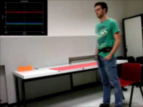
Follow this link to see a video of the 6 activities recorded in the experiment with one of the participants:
I will be using an LSTM on the data to learn (as a cellphone attached on the waist) to recognise the type of activity that the user is doing.
The sensor signals (accelerometer and gyroscope) were pre-processed by applying noise filters and then sampled in fixed-width sliding windows of 2.56 sec and 50% overlap (128 readings/window). The sensor acceleration signal, which has gravitational and body motion components, was separated using a Butterworth low-pass filter into body acceleration and gravity. The gravitational force is assumed to have only low frequency components, therefore a filter with 0.3 Hz cutoff frequency was used. From each window, a vector of features was obtained by calculating variables from the time and frequency domain.
Scroll on! Nice visuals awaits.
# All Includes

import numpy as np
import matplotlib
import matplotlib.pyplot as plt
import tensorflow as tf
from tensorflow.models.rnn import rnn, rnn_cell
from sklearn import metrics

import os
# Useful Constants
# Those are separate normalised input features for the neural network
INPUT_SIGNAL_TYPES = [
"body_acc_x_",
"body_acc_y_",
"body_acc_z_",
"body_gyro_x_",
"body_gyro_y_",
"body_gyro_z_",
"total_acc_x_",
"total_acc_y_",
"total_acc_z_"
]
# Output classes to learn how to classify
LABELS = [
"WALKING",
"WALKING_UPSTAIRS",
"WALKING_DOWNSTAIRS",
"SITTING",
"STANDING",
"LAYING"
] # Note: Linux bash commands start with a "!" inside those "ipython notebook" cells
DATA_PATH = "data/"
!pwd && ls
os.chdir(DATA_PATH)
!pwd && ls
!python download_dataset.py
!pwd && ls
os.chdir("..")
!pwd && ls
DATASET_PATH = DATA_PATH + "UCI HAR Dataset/"
print("\n" + "Dataset is now located at: " + DATASET_PATH)/home/gui/Documents/GIT/LSTM-Human-Activity-Recognition
data LSTM_files LSTM.ipynb README.md
/home/gui/Documents/GIT/LSTM-Human-Activity-Recognition/data
download_dataset.py __MACOSX source.txt UCI HAR Dataset UCI HAR Dataset.zip
Downloading...
Dataset already downloaded. Did not download twice.
Extracting...
Dataset already extracted. Did not extract twice.
/home/gui/Documents/GIT/LSTM-Human-Activity-Recognition/data
download_dataset.py __MACOSX source.txt UCI HAR Dataset UCI HAR Dataset.zip
/home/gui/Documents/GIT/LSTM-Human-Activity-Recognition
data LSTM_files LSTM.ipynb README.md
Dataset is now located at: data/UCI HAR Dataset/
TRAIN = "train/"
TEST = "test/"


# Load "X" (the neural network's training and testing inputs)

def load_X(X_signals_paths):
    X_signals = []

    for signal_type_path in X_signals_paths:
        file = open(signal_type_path, 'rb')
        # Read dataset from disk, dealing with text files' syntax
        X_signals.append(
            [np.array(serie, dtype=np.float32) for serie in [
                row.replace('  ', ' ').strip().split(' ') for row in file
            ]]
        )
        file.close()

    return np.transpose(np.array(X_signals), (1, 2, 0))

X_train_signals_paths = [
    DATASET_PATH + TRAIN + "Inertial Signals/" + signal + "train.txt" for signal in INPUT_SIGNAL_TYPES
]
X_test_signals_paths = [
    DATASET_PATH + TEST + "Inertial Signals/" + signal + "test.txt" for signal in INPUT_SIGNAL_TYPES
]

X_train = load_X(X_train_signals_paths)
X_test = load_X(X_test_signals_paths)


# Load "y" (the neural network's training and testing outputs)

def load_y(y_path):
    file = open(y_path, 'rb')
    # Read dataset from disk, dealing with text file's syntax
    y_ = np.array(
        [elem for elem in [
            row.replace('  ', ' ').strip().split(' ') for row in file
        ]],
        dtype=np.int32
    )
    file.close()

    # Substract 1 to each output class for friendly 0-based indexing
    return y_ - 1

y_train_path = DATASET_PATH + TRAIN + "y_train.txt"
y_test_path = DATASET_PATH + TEST + "y_test.txt"

y_train = load_y(y_train_path)
y_test = load_y(y_test_path)Here are some core parameter definitions for the training.
The whole neural network's structure could be summarised by enumerating those parameters and the fact an LSTM is used.
# Input Data

training_data_count = len(X_train)  # 7352 training series (with 50% overlap between each serie)
test_data_count = len(X_test)  # 2947 testing series
n_steps = len(X_train[0])  # 128 timesteps per series
n_input = len(X_train[0][0])  # 9 input parameters per timestep


# LSTM Neural Network's internal structure

n_hidden = 28 # Hidden layer num of features
n_classes = 6 # Total classes (should go up, or should go down)


# Training

learning_rate = 0.0015
training_iters = training_data_count * 100  # Loop 100 times on the dataset, for a total of 7352000 iterations
batch_size = 1500
display_iter = 15000  # To show test set accuracy during training


# Some debugging info

print "Some useful info to get an insight on dataset's shape and normalisation:"
print "(X shape, y shape, every X's mean, every X's standard deviation)"
print (X_test.shape, y_test.shape, np.mean(X_test), np.std(X_test))
print "The dataset is therefore properly normalised, as expected, but not yet one-hot encoded."
Some useful info to get an insight on dataset's shape and normalisation:
(X shape, y shape, every X's mean, every X's standard deviation)
((2947, 128, 9), (2947, 1), 0.099139921, 0.39567086)
The dataset is therefore properly normalised, as expected, but not yet one-hot encoded.
def LSTM_RNN(_X, _istate, _weights, _biases):
    # Function returns a tensorflow LSTM (RNN) artificial neural network from given parameters.
    # Note, some code of this notebook is inspired from an slightly different
    # RNN architecture used on another dataset:
    # https://tensorhub.com/aymericdamien/tensorflow-rnn

    # (NOTE: This step could be greatly optimised by shaping the dataset once
    # input shape: (batch_size, n_steps, n_input)
    _X = tf.transpose(_X, [1, 0, 2])  # permute n_steps and batch_size
    # Reshape to prepare input to hidden activation
    _X = tf.reshape(_X, [-1, n_input]) # (n_steps*batch_size, n_input)

    # Linear activation
    _X = tf.matmul(_X, _weights['hidden']) + _biases['hidden']
    # Define a lstm cell with tensorflow
    lstm_cell = rnn_cell.BasicLSTMCell(n_hidden, forget_bias=1.0)
    # Split data because rnn cell needs a list of inputs for the RNN inner loop
    _X = tf.split(0, n_steps, _X) # n_steps * (batch_size, n_hidden)

    # Get lstm cell output
    outputs, states = rnn.rnn(lstm_cell, _X, initial_state=_istate)

    # Linear activation
    # Get inner loop last output
    return tf.matmul(outputs[-1], _weights['out']) + _biases['out']


def extract_batch_size(_train, step, batch_size):
    # Function to fetch a "batch_size" amount of data from "(X|y)_train" data.

    shape = list(_train.shape)
    shape[0] = batch_size
    batch_s = np.empty(shape)

    for i in range(batch_size):
        # Loop index
        index = ((step-1)*batch_size + i) % len(_train)
        batch_s[i] = _train[index]

    return batch_s


def one_hot(y_):
    # Function to encode output labels from number indexes
    # e.g.: [[5], [0], [3]] --> [[0, 0, 0, 0, 0, 1], [1, 0, 0, 0, 0, 0], [0, 0, 0, 1, 0, 0]]

    y_ = y_.reshape(len(y_))
    n_values = np.max(y_) + 1
return np.eye(n_values)[np.array(y_, dtype=np.int32)] # Returns FLOATS# Graph input/output
x = tf.placeholder("float", [None, n_steps, n_input])
istate = tf.placeholder("float", [None, 2*n_hidden]) #state & cell => 2x n_hidden
y = tf.placeholder("float", [None, n_classes])
# Graph weights
weights = {
'hidden': tf.Variable(tf.random_normal([n_input, n_hidden])), # Hidden layer weights
'out': tf.Variable(tf.random_normal([n_hidden, n_classes]))
}
biases = {
'hidden': tf.Variable(tf.random_normal([n_hidden])),
'out': tf.Variable(tf.random_normal([n_classes]))
}
pred = LSTM_RNN(x, istate, weights, biases)
# Loss, optimizer and evaluation
cost = tf.reduce_mean(tf.nn.softmax_cross_entropy_with_logits(pred, y)) # Softmax loss
optimizer = tf.train.AdamOptimizer(learning_rate=learning_rate).minimize(cost) # Adam Optimizer
correct_pred = tf.equal(tf.argmax(pred,1), tf.argmax(y,1))
accuracy = tf.reduce_mean(tf.cast(correct_pred, tf.float32))# To keep track of training's performance
test_losses = []
test_accuracies = []
train_losses = []
train_accuracies = []
# Launch the graph
sess = tf.InteractiveSession(config=tf.ConfigProto(log_device_placement=True))
init = tf.initialize_all_variables()
sess.run(init)
# Perform Training steps with "batch_size" iterations at each loop
step = 1
while step * batch_size <= training_iters:
batch_xs = extract_batch_size(X_train, step, batch_size)
batch_ys = one_hot(extract_batch_size(y_train, step, batch_size))
# Fit training using batch data
_, loss, acc = sess.run(
[optimizer, cost, accuracy],
feed_dict={
x: batch_xs,
y: batch_ys,
istate: np.zeros((batch_size, 2*n_hidden))
}
)
train_losses.append(loss)
train_accuracies.append(acc)
# Evaluate network only at some steps for faster training:
if (step*batch_size % display_iter == 0) or (step == 1) or (step * batch_size > training_iters):
# To not spam console, show training accuracy/loss in this "if"
print "Iter " + str(step*batch_size) + \
", Batch Loss= " + "{:.6f}".format(loss) + \
", Accuracy= " + "{}".format(acc)
# Evaluation on the test set (no learning made here - just evaluation for diagnosis)
loss, acc = sess.run(
[cost, accuracy],
feed_dict={
x: X_test,
y: one_hot(y_test),
istate: np.zeros((len(X_test), 2*n_hidden))
}
)
test_losses.append(loss)
test_accuracies.append(acc)
print "TEST SET DISPLAY STEP: " + \
"Batch Loss= {}".format(loss) + \
", Accuracy= " + "{}".format(acc)
step += 1
print "Optimization Finished!"
# Accuracy for test data
one_hot_predictions, accuracy, final_loss = sess.run(
[pred, accuracy, cost],
feed_dict={
x: X_test,
y: one_hot(y_test),
istate: np.zeros((len(X_test), 2*n_hidden))
}
)
test_losses.append(final_loss)
test_accuracies.append(accuracy)
print "FINAL RESULT: " + \
"Batch Loss= {}".format(final_loss) + \
", Accuracy= " + "{}".format(accuracy)Iter 1500, Batch Loss= 3.497532, Accuracy= 0.167333334684
TEST SET DISPLAY STEP: Batch Loss= 2.93614697456, Accuracy= 0.200882256031
Iter 15000, Batch Loss= 1.597702, Accuracy= 0.45666667819
TEST SET DISPLAY STEP: Batch Loss= 1.55875110626, Accuracy= 0.38581609726
Iter 30000, Batch Loss= 1.238804, Accuracy= 0.499333322048
TEST SET DISPLAY STEP: Batch Loss= 1.22680544853, Accuracy= 0.504580914974
Iter 45000, Batch Loss= 0.954462, Accuracy= 0.663999974728
TEST SET DISPLAY STEP: Batch Loss= 1.02884912491, Accuracy= 0.61418390274
Iter 60000, Batch Loss= 0.804594, Accuracy= 0.680000007153
TEST SET DISPLAY STEP: Batch Loss= 0.924499809742, Accuracy= 0.623685121536
Iter 75000, Batch Loss= 0.698102, Accuracy= 0.719333350658
TEST SET DISPLAY STEP: Batch Loss= 0.794336855412, Accuracy= 0.666779756546
Iter 90000, Batch Loss= 0.608659, Accuracy= 0.757333338261
TEST SET DISPLAY STEP: Batch Loss= 0.723006248474, Accuracy= 0.70105189085
Iter 105000, Batch Loss= 0.507658, Accuracy= 0.817333340645
TEST SET DISPLAY STEP: Batch Loss= 0.690091133118, Accuracy= 0.737699329853
Iter 120000, Batch Loss= 0.424661, Accuracy= 0.85799998045
TEST SET DISPLAY STEP: Batch Loss= 0.674829542637, Accuracy= 0.764506280422
Iter 135000, Batch Loss= 0.327075, Accuracy= 0.90066665411
TEST SET DISPLAY STEP: Batch Loss= 0.668574094772, Accuracy= 0.781472682953
Iter 150000, Batch Loss= 0.288192, Accuracy= 0.910000026226
TEST SET DISPLAY STEP: Batch Loss= 0.626025915146, Accuracy= 0.782829999924
Iter 165000, Batch Loss= 0.406867, Accuracy= 0.82266664505
TEST SET DISPLAY STEP: Batch Loss= 0.534764289856, Accuracy= 0.818120121956
Iter 180000, Batch Loss= 0.350908, Accuracy= 0.851333320141
TEST SET DISPLAY STEP: Batch Loss= 0.513215303421, Accuracy= 0.820834755898
Iter 195000, Batch Loss= 0.298054, Accuracy= 0.864000022411
TEST SET DISPLAY STEP: Batch Loss= 0.499158024788, Accuracy= 0.829996585846
Iter 210000, Batch Loss= 0.273907, Accuracy= 0.854666650295
TEST SET DISPLAY STEP: Batch Loss= 0.506343245506, Accuracy= 0.834747195244
Iter 225000, Batch Loss= 0.242510, Accuracy= 0.875333309174
TEST SET DISPLAY STEP: Batch Loss= 0.511559724808, Accuracy= 0.839837133884
Iter 240000, Batch Loss= 0.139401, Accuracy= 0.96266669035
TEST SET DISPLAY STEP: Batch Loss= 0.483630269766, Accuracy= 0.844587743282
Iter 255000, Batch Loss= 0.112158, Accuracy= 0.974666655064
TEST SET DISPLAY STEP: Batch Loss= 0.460559636354, Accuracy= 0.855785548687
Iter 270000, Batch Loss= 0.124294, Accuracy= 0.975333333015
TEST SET DISPLAY STEP: Batch Loss= 0.470139116049, Accuracy= 0.854088902473
Iter 285000, Batch Loss= 0.103742, Accuracy= 0.977333307266
TEST SET DISPLAY STEP: Batch Loss= 0.442456573248, Accuracy= 0.862911462784
Iter 300000, Batch Loss= 0.095325, Accuracy= 0.979333341122
TEST SET DISPLAY STEP: Batch Loss= 0.430220544338, Accuracy= 0.869697988033
Iter 315000, Batch Loss= 0.076378, Accuracy= 0.985333323479
TEST SET DISPLAY STEP: Batch Loss= 0.485659360886, Accuracy= 0.862572133541
Iter 330000, Batch Loss= 0.140580, Accuracy= 0.9646666646
TEST SET DISPLAY STEP: Batch Loss= 0.41461867094, Accuracy= 0.877502560616
Iter 345000, Batch Loss= 0.153887, Accuracy= 0.94866669178
TEST SET DISPLAY STEP: Batch Loss= 0.415001064539, Accuracy= 0.878520548344
Iter 360000, Batch Loss= 0.150718, Accuracy= 0.946666657925
TEST SET DISPLAY STEP: Batch Loss= 0.410178214312, Accuracy= 0.883949756622
Iter 375000, Batch Loss= 0.163540, Accuracy= 0.938666641712
TEST SET DISPLAY STEP: Batch Loss= 0.397105753422, Accuracy= 0.891754329205
Iter 390000, Batch Loss= 0.154012, Accuracy= 0.939999997616
TEST SET DISPLAY STEP: Batch Loss= 0.400521725416, Accuracy= 0.887682378292
Iter 405000, Batch Loss= 0.108920, Accuracy= 0.95733332634
TEST SET DISPLAY STEP: Batch Loss= 0.401270329952, Accuracy= 0.892772316933
Iter 420000, Batch Loss= 0.104911, Accuracy= 0.955999970436
TEST SET DISPLAY STEP: Batch Loss= 0.395263999701, Accuracy= 0.894468963146
Iter 435000, Batch Loss= 0.105534, Accuracy= 0.951333343983
TEST SET DISPLAY STEP: Batch Loss= 0.392485201359, Accuracy= 0.894808292389
Iter 450000, Batch Loss= 0.141352, Accuracy= 0.938000023365
TEST SET DISPLAY STEP: Batch Loss= 0.405577093363, Accuracy= 0.887343049049
Iter 465000, Batch Loss= 0.148221, Accuracy= 0.931999981403
TEST SET DISPLAY STEP: Batch Loss= 0.393891453743, Accuracy= 0.890057682991
Iter 480000, Batch Loss= 0.127158, Accuracy= 0.937333345413
TEST SET DISPLAY STEP: Batch Loss= 0.393162339926, Accuracy= 0.891414999962
Iter 495000, Batch Loss= 0.089967, Accuracy= 0.969333350658
TEST SET DISPLAY STEP: Batch Loss= 0.389132201672, Accuracy= 0.892772316933
Iter 510000, Batch Loss= 0.086796, Accuracy= 0.975333333015
TEST SET DISPLAY STEP: Batch Loss= 0.384798914194, Accuracy= 0.892093658447
Iter 525000, Batch Loss= 0.082901, Accuracy= 0.97866666317
TEST SET DISPLAY STEP: Batch Loss= 0.384688735008, Accuracy= 0.899219572544
Iter 540000, Batch Loss= 0.157561, Accuracy= 0.930666685104
TEST SET DISPLAY STEP: Batch Loss= 0.402176290751, Accuracy= 0.887682378292
Iter 555000, Batch Loss= 0.183808, Accuracy= 0.919333338737
TEST SET DISPLAY STEP: Batch Loss= 0.391167700291, Accuracy= 0.896844267845
Iter 570000, Batch Loss= 0.168330, Accuracy= 0.926666676998
TEST SET DISPLAY STEP: Batch Loss= 0.38873809576, Accuracy= 0.897183597088
Iter 585000, Batch Loss= 0.165021, Accuracy= 0.928666651249
TEST SET DISPLAY STEP: Batch Loss= 0.387221038342, Accuracy= 0.895486950874
Iter 600000, Batch Loss= 0.147256, Accuracy= 0.931333363056
TEST SET DISPLAY STEP: Batch Loss= 0.370691657066, Accuracy= 0.899558901787
Iter 615000, Batch Loss= 0.080325, Accuracy= 0.973333358765
TEST SET DISPLAY STEP: Batch Loss= 0.385037720203, Accuracy= 0.902952134609
Iter 630000, Batch Loss= 0.070145, Accuracy= 0.980000019073
TEST SET DISPLAY STEP: Batch Loss= 0.390854179859, Accuracy= 0.898201584816
Iter 645000, Batch Loss= 0.082961, Accuracy= 0.972666680813
TEST SET DISPLAY STEP: Batch Loss= 0.394806742668, Accuracy= 0.901255488396
Iter 660000, Batch Loss= 0.079043, Accuracy= 0.97000002861
TEST SET DISPLAY STEP: Batch Loss= 0.391038626432, Accuracy= 0.901255488396
Iter 675000, Batch Loss= 0.081615, Accuracy= 0.96266669035
TEST SET DISPLAY STEP: Batch Loss= 0.413295030594, Accuracy= 0.887343049049
Iter 690000, Batch Loss= 0.054776, Accuracy= 0.994000017643
TEST SET DISPLAY STEP: Batch Loss= 0.405757367611, Accuracy= 0.891075670719
Iter 705000, Batch Loss= 0.117449, Accuracy= 0.967333316803
TEST SET DISPLAY STEP: Batch Loss= 0.374152183533, Accuracy= 0.902612805367
Iter 720000, Batch Loss= 0.123223, Accuracy= 0.952666640282
TEST SET DISPLAY STEP: Batch Loss= 0.394488096237, Accuracy= 0.898880243301
Iter 735000, Batch Loss= 0.116774, Accuracy= 0.953999996185
TEST SET DISPLAY STEP: Batch Loss= 0.38473045826, Accuracy= 0.898880243301
Optimization Finished!
FINAL RESULT: Batch Loss= 0.38473045826, Accuracy= 0.898880243301
Okay, let's do it simply in the notebook for now
# (Inline plots: )
%matplotlib inline

font = {
    'family' : 'Bitstream Vera Sans',
    'weight' : 'bold',
    'size'   : 18
}
matplotlib.rc('font', **font)

width = 12
height = 12
plt.figure(figsize=(width, height))

indep_train_axis = np.array(range(batch_size, (len(train_losses)+1)*batch_size, batch_size))
plt.plot(indep_train_axis, np.array(train_losses),     "b--", label="Train losses")
plt.plot(indep_train_axis, np.array(train_accuracies), "g--", label="Train accuracies")

indep_test_axis = np.array(range(batch_size, len(test_losses)*display_iter, display_iter)[:-1] + [training_iters])
plt.plot(indep_test_axis, np.array(test_losses),     "b-", label="Test losses")
plt.plot(indep_test_axis, np.array(test_accuracies), "g-", label="Test accuracies")

plt.title("Training session's progress over iterations")
plt.legend(loc='upper right', shadow=True)
plt.ylabel('Training Progress (Loss or Accuracy values)')
plt.xlabel('Training iteration')

plt.show()
# Results

predictions = one_hot_predictions.argmax(1)

print "Testing Accuracy: {}%".format(100*accuracy)

print ""
print "Precision: {}%".format(100*metrics.precision_score(y_test, predictions, average="weighted"))
print "Recall: {}%".format(100*metrics.recall_score(y_test, predictions, average="weighted"))
print "f1_score: {}%".format(100*metrics.f1_score(y_test, predictions, average="weighted"))

print ""
print "Confusion Matrix:"
confusion_matrix = metrics.confusion_matrix(y_test, predictions)
print confusion_matrix
normalised_confusion_matrix = np.array(confusion_matrix, dtype=np.float32)/np.sum(confusion_matrix)*100

print ""
print "Confusion matrix (normalised to % of total test data):"
print normalised_confusion_matrix
print ("Note: training and testing data is not equally distributed amongst classes, "
       "so it is normal that more than a 6th of the data is correctly classifier in the last category.")

# Plot Results:
width = 12
height = 12
plt.figure(figsize=(width, height))
plt.imshow(
    normalised_confusion_matrix,
    interpolation='nearest',
    cmap=plt.cm.rainbow
)
plt.title("Confusion matrix \n(normalised to % of total test data)")
plt.colorbar()
tick_marks = np.arange(n_classes)
plt.xticks(tick_marks, LABELS, rotation=90)
plt.yticks(tick_marks, LABELS)
plt.tight_layout()
plt.ylabel('True label')
plt.xlabel('Predicted label')
plt.show()
Testing Accuracy: 89.8880243301%
Precision: 89.933405934%
Recall: 89.888021717%
f1_score: 89.8191732334%
Confusion Matrix:
[[453 10 33 0 0 0]
[ 1 446 24 0 0 0]
[ 6 6 408 0 0 0]
[ 1 25 0 384 81 0]
[ 1 19 1 89 422 0]
[ 0 1 0 0 0 536]]
Confusion matrix (normalised to % of total test data):
[[ 15.37156391 0.33932811 1.11978292 0. 0. 0. ]
[ 0.03393281 15.13403511 0.8143875 0. 0. 0. ]
[ 0.20359688 0.20359688 13.84458828 0. 0. 0. ]
[ 0.03393281 0.84832031 0. 13.0302 2.74855804 0. ]
[ 0.03393281 0.64472347 0.03393281 3.02002048 14.31964684 0. ]
[ 0. 0.03393281 0. 0. 0. 18.18798828]]
Note: training and testing data is not equally distributed amongst classes, so it is normal that more than a 6th of the data is correctly classifier in the last category.

sess.close()Outstandingly, the accuracy is of 89.888%!
This means that the neural networks is almost always able to correctly identify the movement type! Remember, the phone is attached on the waist and each series to classify has just a 128 sample window of two internal sensors (a.k.a. 2.56 seconds at 50 FPS), so those predictions are extremely accurate.
I specially did not expect such good results for guessing between "WALKING" "WALKING_UPSTAIRS" and "WALKING_DOWNSTAIRS" as a cellphone. Tought, it is still possible to see a little cluster on the matrix between those 3 classes. This is great.
It is also possible to see that it was hard to do the difference between "SITTING" and "STANDING". Those are seemingly almost the same thing from the point of view of a device placed at waist level.
The dataset is described on the UCI Machine Learning Repository:
Davide Anguita, Alessandro Ghio, Luca Oneto, Xavier Parra and Jorge L. Reyes-Ortiz. A Public Domain Dataset for Human Activity Recognition Using Smartphones. 21th European Symposium on Artificial Neural Networks, Computational Intelligence and Machine Learning, ESANN 2013. Bruges, Belgium 24-26 April 2013.
# Let's convert this notebook to a README as the GitHub project's title page:
!jupyter nbconvert --to markdown LSTM.ipynb
!mv LSTM.md README.md
[NbConvertApp] Converting notebook LSTM.ipynb to markdown
[NbConvertApp] Support files will be in LSTM_files/
[NbConvertApp] Making directory LSTM_files
[NbConvertApp] Making directory LSTM_files
[NbConvertApp] Writing 24317 bytes to LSTM.md

