summuk / eeg Goto Github PK

#Pattern Recognition of Nonlinear Dynamic Systems

The human brain is a very complex structure. It has almost hundred billion neurons and at least hundred trillion connections[10]. This enormous neural network and the complex processing makes it capable of recognizing objects around us a trivial task. Human recognition of temporal patterns is a coordinated process. In this process patterns of data distributed over time can be recognized, represented and classified. What makes human recognition more interesting is the pace from detecting temporal patterns, extracting of features and final pattern matching[19]. Implementing this functionality artificially is a daunting task, but science has developed tools & techniques to realize the goal. Pattern recognition has wide range of applications today. Face recognition, speech recognition, hand writing classification, medical diagnosis to name a few. Even though pattern recognition applications varies widely, the approach to achieve the final goal is same. It starts by data acquisition and cleaning of data. Then comes feature extraction and finally based on the extracted features the data is classified. Figure 38 represents information processing pipeline of pattern recognition where data travels from environment to the classifier through different layers. 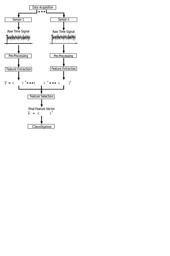Figure 38: Flowchart of the pattern recognition experiment through various stages[93]. Nonlinear dynamical signals pattern recognition and classification are discussed in the chapter. Many of the previous works deal with pattern recognition and classification of static patterns but little attention have been given into learning temporal patterns showing chaotic nature. A novel method for classification of nonlinear dynamic patterns is proposed in the chapter, the method deploys statistically considerable number of labeled data for each of the classes to a classifier for pattern recognition. Two types of nonlinear dynamical signals are used, artificial and real world. Artificial signals include chaotic state signals of Chen’s, Lorenz, and Rossler’s system. EEG signals are the real world signal used for the pattern recognition study. Pattern recognition and classification of EEG during cognitive tasks and relating to mental state are successfully done in previous works. But not a lot of effort has been put to recognize and classify EEG patterns during emotional tasks related to traumatic memories. Individual studies by researchers have shown that the focused guided imagery and tailored meditation helps to develop greater inter-regional brain activity correlation on the right hemisphere of brain[94]. A traditional healing therapy for PTSD subjects are developed by a nonverbal replay of the traumatic memories through their mind. The customized regression protocol is known as “Soul Retrieval”, developed by Dr. Jane Simington[95]. It is customized for each subject and uses guided imagery to invite healing. Different physiological measurements are taken during this experiment including EEG, ECG, blood hemoglobin level, brain hemispherical oxygenation level to evaluate the effectiveness of the newly developed method. Pattern recognition of EEG data is done on the two important patterns collected during the experiment. The goal of this pattern recognition approach is to identify the EEG pattern changes in the prefrontal cortex of the brain that is responsible for short term memories and identify it during the soul retrieval process.

EEG data are recoded during two mental states from each subjects (i) EEG data recorded during guided imagery test known as hyperarousal pattern (ii) EEG signal recorded during a baseline task eyes open. Statistical time-frequency domain feature extraction method, wavelet transform is applied on the data. The proposed method differentiates itself from the previous approaches in three ways.

First, this work studies about the statistical features of nonlinear dynamical systems in time domain, and in time-frequency domain. Hence the most efficient feature set can be identified and extracted from channels based on the dimensionality of the system.

Second, the pattern recognition method uses different classifiers employing a variety of machine learning algorithms with a special focus on neural network algorithms for pattern classification. These machine learning algorithm-based classifiers have an established evaluation criterion to classify patterns. Thus, the proposed method outperforms deterministic algorithms in classification of patterns.

Third, several studies skipped feature normalization and or feature selection steps when doing feature extraction for pattern recognition. And, many studies used simple cognitive tasks that wasn’t powerful enough to activate correlative neuronal structures for detectable potential. Also, some studies failed to ensure that the results of classifier are over fitted or the classifiers are just remembering the training set. These limitations are effectively covered in the proposed study by employing a powerful and mental task, and by deploying feature normalization and cross validation of the classifier during training and evaluation.

5.1 Proposed Pattern Recognition Model for Nonlinear Dynamic Systems The first stage of pattern recognition task is data acquisition. It is done by sensors which give raw data in terms of velocity, power, current, voltage or vibration values. The data needs preprocessing to get rid of noise and other unwanted artifacts. The raw time domain values which are often nonstationary are submitted for statistical processing like Time domain analysis, Fourier transform, Wavelet Transform or any other method that provides stationary values. This process is known as feature extraction in the measurement level[96]. Once features are extracted their distribution is verified before applying any normalization method. All extracted features are normalized so that the features measured on different scales are brought to a common scale. The process of retaining only a relatively small number of features which additionally are the most discriminative ones is known as feature selection. Once feature selection is done feature dataset is optimized and is ready to be fed to the classifiers. A wide variety of classifiers are available to distinguish the one class of data from another. The classifier is chosen based on the purpose and the nature of data, for example CNN is good for image classification while RNN/LSTM is good for nonlinear pattern classification. Apart from that there are several conventional statistical classifiers which we will see later. Data is divided into training and testing set before classification and the classifier is trained on training dataset which is labelled, and the performance is evaluated. Once trained successfully the classifier is used to classify the test data labelled but unknown to the classifier. A unique method for feature extraction is proposed in this study where the features extracted are small and efficient to ensure classification high accuracy. Since this study focusses on identifying specific EEG pattern during a mental task from several people, as a first step a two class classification is experimented. The difficulty as well as data requirements for training ANN is reduced greatly for a two-class classification task compared to a multi-class problem. Lorenz, Rossler and Chen as well as EEG patterns are formulated into a two-class classification task and evaluated. Figure 39 summarizes the proposed pattern recognition scheme which comprises of following steps:

Feature Extraction Time domain feature extraction Measurement of RMS, Peak-peak value, Peak value, Crest factor and Kurtosis. Time-Frequency domain feature extraction The DWT is employed and the signal is decomposed in corresponding energy sub-bands. The relative energy of each sub-bands are then computed. Feature Visualization Check the distribution of the features using a normal probability and histogram plots. Feature Standardization The extracted features are standardized with zero mean and unit variance. Feature Classification Classification of the selected features using Decision Tree, KNN, SVM, MLP and LSTM. 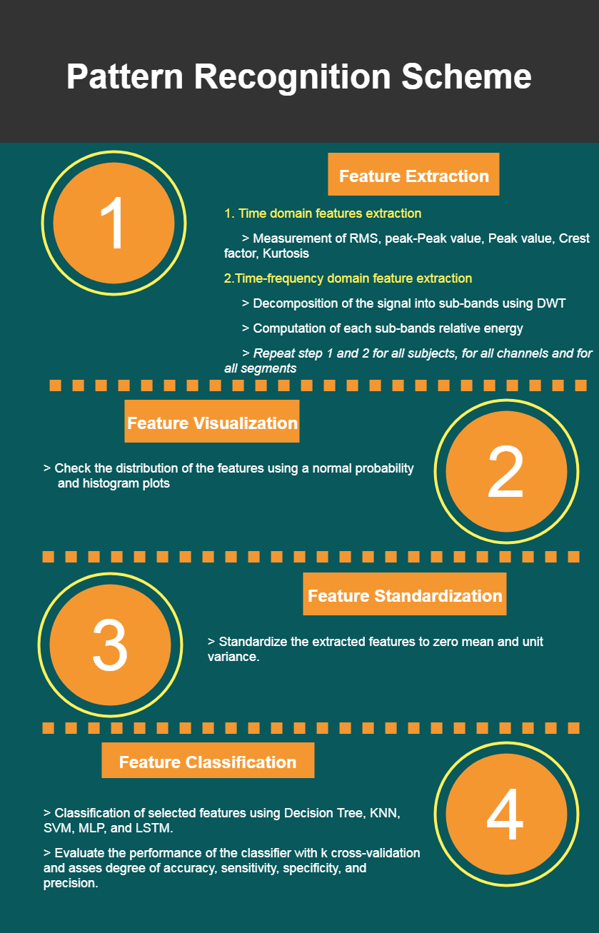Figure 39: Proposed method for EEG signals feature extraction and classification. 5.1.1 Feature Extraction The performance of pattern recognition systems is influenced by the (i) amount of data (ii) pattern recognition approach used. The total number of samples representing data depends on two factors namely, sampling frequency and duration of data acquisition. Pattern recognition has been conventionally studied following the main approaches like statistical, temporal, structural, neural network and fuzzy. Among these statistical approach has been mostly used for data analysis and classification [97]. In our study data is not a limiting factor hence we will study about pattern recognition approach followed. 5.1.1.1 Statistical Approach

Statistical model pattern recognition needs patterns to be described in terms of features. Features are chosen in such a way that different patterns occupy non-overlapping feature space. Non overlapping feature space represents the probabilistic nature of the information we access from the data as well as the representation of such feature to a classifier model[98]. This results in feature spaces forming recognizable clusters. After analyzing the probability distribution of the features of the pattern, decision boundaries are determined[99]. Preprocessing operations are done on patterns to make them suitable for training and after analyzing preprocessed data, features are selected. To evaluate whether the model has learned to classify features instead of just remembering the training vector, a test pattern is fed. Once this process is found satisfactory the model can be used for classification of new patterns without further training. One of the advantages of the statistical model is that system becomes noise insensitive and for noisy patterns this is an ideal solution. Based on whether unsupervised or supervised method is employed statistical technique is categorized as Discriminant Analysis and Principal Component Analysis. Discriminant analysis is a supervised technique where linear combination of the feature is used to perform the classification operation. Linear Discriminant Analysis, Fisher Discriminant Analysis, Null- LDA and two dimensional LDA are some example of Linear Discriminant Analysis. Principal Component Analysis is a multi-element unsupervised technique used for dimensionality reduction. Common statistical feature extraction techniques include Fourier Transform in frequency domain, Short term Fourier Transform, and Wavelet transform in Time-Frequency domain. 5.1.1.1.1 Time Domain Features The raw data we have for pattern recognition are discretized signals and some discriminative information in the form of statistical parameters can be gained from it. Time domain features are temporal information which can be extracted from the time series. This gives a great deal of insight into the shape of the patterns, nonlinear dynamics, different peak values and recurring patterns. Extracting this information helps in training the classifier models on general difference in shapes of data. The features of nonlinear dynamical systems are temporal in nature, it means chaotic patterns vary with respect to time. A variety of features representing different states of the nonlinear dynamical systems is used for feature extraction. We present five-time domain features below. Root Mean Square (RMS) RMS is one of the basic measurements of a time domain signal which describes the energy of the signal. It is defined as the square root of the average squared value of the signal and call also be called as the normalized energy of signal[96]. It can be mathematically defined as: RMS=√(1/n ∑_(i=0)^(n-1)▒s_i^2 ) (57) It can be used for fault detection or set off an alarm when the RMS value surpasses a certain threshold. RMS also gives an idea of the general range of signal power and this is an important feature as it helps classifier to distinguish signals by average power. Figure 40 shows the difference in the Lorenz and Rossler’s system and their corresponding RMS values.

Peak to Peak Value (PP) Peal to Peak is an important measurement of a signal, if you consider a semantically coherent sampling interval the peak to peak value represents the amplitude spread of a signal[96]. It is calculated by the difference in the amplitude between peak and trough of a signal. It is represented as: Pv=1/2 (58) Peak to Peak value also gives an idea of the general envelope of the signal and this is an important feature as it helps classifier to distinguish signals by amplitude. Figure 41 shows the difference in the Lorenz and Rossler’s system and their corresponding RMS values.

Figure 41: Lorenz and Rossler’s system with their Peak -Peak value of signals Peak value

Peak value of a signal is the maximum amplitude of a signal compared to a reference level s_ref which is generally zero[96]. This can be calculated by taking the difference between the reference level and signal amplitude. This can be mathematically expressed as follows: Pv=1/2 (59)
Often peak value is used in conjunction with other statistical parameters, for instance the peak to average or peak to median. Figure 42 shows the difference in the Lorenz and Rossler’s system and their corresponding peak values.

Figure 42: Lorenz and Rossler’s system with their Peak value of signals Crest Factor Crest factor is the measure of spikiness of the signal[96]. It can be calculated by dividing the peak value by the RMS of the signal. It can be mathematically expressed as: CF=(1/2 (〖max〗_(i=0)^(n-1) s_i-s_ref ))/RMS (60) CF is also known as peak to average ratio or peak to average power ratio. It is used to characterize signals containing repetitive impulses in addition to a lower level continuous signal. The modulus of signal should be used in calculus.

Kurtosis Kurtosis is a distribution function for measurement of spikiness of a signal[96]. The purpose of this measurement is similar to crest factor but in a higher order than the crest factor. It can be expressed as the ratio of fourth moment around the mean and the square of the variance. Considering that there are n samples of signal from s_1 to s_n. Kurtosis can be calculated as: K=-3+(1/n ∑_(i=0)^(n-1)▒(s_i-s ̅ )^4 )/([1/n ∑_(i=0)^(n-1)▒〖(s_i-s ̅ )^2 ]^2 〗) (61) where S ̅ denotes the estimated expected value (average) of the signal. Kurtosis describes how peaked or float the distribution is. If a signal contains sharp peaks with a higher value, then its distribution function will be sharper. The features are extracted for each class of signal, for all channels and for all segments. The extracted features are stored into a feature vector for each class with their target vectors and proceed further to visualization and standardization. 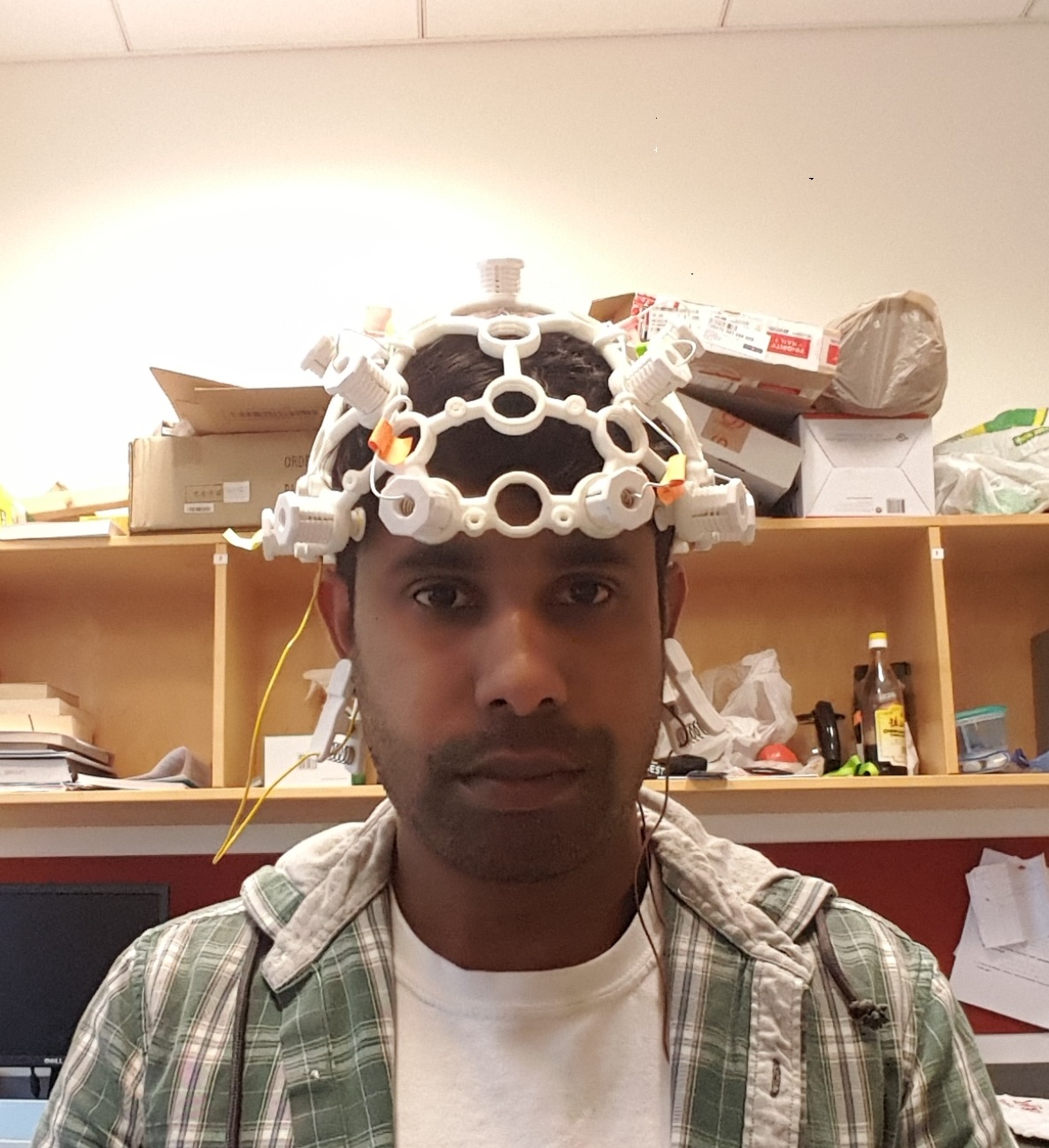Figure 56: ULTRACORTEX MARK IV headware after assembling 5.1.1.1.2 Time- Frequency Domain Features Nonlinear dynamical signal analysis are done on time domain and frequency domain. To gain knowledge about the spectral properties of the signals, frequency analysis is performed. Since the collected signals may contain noise and other artifacts, for preprocessing it is important to gain information of the frequency content of the signal. This information can be used to filter the unwanted noise signals and make signal more robust. Frequency information of nonlinear dynamical signals are very important because the band derivatives holds important information useful for classification. There are various techniques to extract frequency information from signals. Fourier transform is a tool used to perform frequency analysis, which decomposes the signal into additive sine and cosine terms in the complex domain. Even though the phase angle of the complex domain function is a valuable source of information, the magnitude part is more important, known as frequency spectrum. Frequency spectrum displays various frequency contents of the underlying signals against its amplitude, it is symmetric and only one half must be kept. One problem with the frequency analysis is that it ignores the temporal information content, i.e., it doesn’t care about when a change in signal power happens and focus just the overall change. For nonlinear dynamical signals, if we want to know about the spectral changes at a particular dynamical state, Fourier transform won’t give a precise information. The information from the signals will be more accurate if we employ some analytic techniques that try to capture frequency content at different time instances. This kind of hybrid representation of signal with changing intensities over time and simultaneously capturing the frequency of patterns is known as time frequency representation. It is particularly effective in nonstationary time series study. There are various time frequency analysis methods like Short Time Fourier Transform (STFT) where multiplies a signal with a window and take Fourier transform of the product[96]. The counterpart of Fourier Transform in time-frequency domain is called Wavelet Transform (WT) [100]. When compared to the STFT which has a fixed window size the WT has the advantage of a flexible resolution in the time and frequency domains. AS in the case of Fourier transform there are various types of Wavelet transform methods, namely CWT, wavelet series expansion, and DWT. For software implementation in digital signal processing the DWT is widely used. In DWT, the signal is decomposed in terms of multiples of wavelet basis function. Several wavelet families have proven to be useful including Haar, Daubechies, Biorthogonal, Coiflets, Symlets, Morlet, etc. Orthogonal dyadic wavelets are the most used in the research owing to it efficient implementation of discrete wavelet transform since the translations and scales are powers of 2. Another perspective of DWT is to look it as a successive high pass and low pass filtering of the input signal with a down sampling rate of 2. The high pass filter which allows high frequency components are the discrete mother wavelet but short in time duration while the low pass filter, a mirror version that allows low frequency components of the input signals are coarse in time. Daubechies wavelet family is used in this study and the mother wavelet is db4 as shown in figure 44. Outputs from the initial high pass filter are known as “approximation coefficients” (A1) and low pass filter as” detailed coefficients” (D1). These are integrated further to reach deeper levels based on the frequency content of the signal and the resolution needed as shown in figure 45. The mother wavelet and scaling can be denoted as follows[96]:

φ_(j,k) (n)=2^((-j)/2 h(2^(-j) n-k) ) (62) φ_(j,k) (n)=2^((-j)/2 g(2^(-j) n-k) ) (63) where m=0,1,2,….,M-1;j=0,1,2,…..J-1;k=0,1,2,…..2j-1;j=5; and M is the length of the signal.

Figure 44: Mother wavelet and scaling function (db4) [101] The approximation coefficients (Ai) and detailed coefficients (Di) at the i_th level are determined as follows[96]: A_i=1/(√M ∑_n▒〖x(n) φ_(j,k) (n) 〗) (64) D_i=1/(√M ∑_n▒〖x(n) φ_(j,k) (n) 〗) (65)
The wavelet energy for each decomposition level (i = 1,…,l) is determined as follows: E_Di=∑_(j=1)^N▒〖|D_ij |^2,i=1,2,…l〗 (66) where l=5, reflects the level of decompositions E_Ai=∑_(j=1)^N▒〖|A_ij |^2,i=l〗 (67) Therefore, from equations (66) and (67), total energy can be defined as: E_Total=(∑_(i=1)^l▒〖E_Di+E_Ai 〗) (68) The normalized energy values represent wavelet energy and can be calculated as follows: E_r=E_j/E_total (69) where E_j=E_Di=1,…5 or E_Ai=5

The above steps can be summarized as follows, the nonlinear dynamic signals are decomposed into sub-band frequencies using the discrete DWT with db4 wavelet up to level 5. Approximated and Detailed coefficients are then computed for each decomposition level. From extracted wavelet coefficients total and relative sub-band energies were then computed using equations (68) and (69). Relative energy is computed for all experimental subjects and from the assigned channel. 5.1.2 Feature Standardization Features are verified before they are fed into the classifier. Features should be the most discriminative ones, non-redundant and distributed normally. This can be verified during feature visualization. Normal probability and histogram plots are used to verify the distribution of feature values. An important preprocessing step for pattern recognition studies is feature standardization. The aim of the standardization is to rescale the features such that they have the properties of a standard normal distribution with a mean of zero and a standard deviation of one. In this study features are standardized according to equation 70: x ´=(x-μ)/σ (70) where x is the original feature value, µ is the mean and σ is the standard deviation of the “features” set, and x ´ is the normalized feature value.

Figure 46: Feature visualization of one sample within dataset using normal probability plot

5.1.3 Feature Classification Standardized features are used for training a classifier. Classifier systems based on different machine learning algorithms are trained and validated over equal number of training samples. During training, a classifier will model an association between classes and corresponding features and become capable of identifying new instances in an unseen test dataset. Once trained, labelled patterns which are unknown to the classifier are used to evaluate the performance of the classifier. To demonstrate the effectiveness proposed pattern recognition in the chapter, following classifiers are employed. Decision Tree Decision trees are used commonly by both programmers and managers (decision nodes). It is a decision support tool that uses a tree like structure and all its possible consequences. They are successfully used for both pattern classification and data mining. Decision trees are produced by algorithms which identify several ways of splitting data set into branch like segments. It starts as an inverted decision tree which starts with a root node at the top of the tree. Several nodes start from the root node called object of analysis and the decision rule is created between nodes and input fields to create the branch or segments. The values of the input field are used to estimate the likely value of the target field which can also be termed as outcome. Decision rules can be derived once a relationship between inputs and targets are found. Once the decision rules are set, and the input fields are fed with unseen observations which are predicted for target values using the decision rules[14].
K Nearest Neighbor Classifier (KNN) If you already have a feature space with enough samples in different classes, and then a new sample came. If you want to classify the newly arrived sample to a class, KNN is the best classifier to help you. It is a method of classifying objects based on the closest training examples on the feature space. KNN is an example-based learning method where the function is only approximated locally, and it is the simplest of machine learning algorithms where object is classified based on the majority decision of its neighbors. The selected k nearest neighbors are known as training samples whose labels and class details are known and is stored in a Euclidean space till a new unlabeled data arrives. Once an unlabeled feature vector or query instance arrives classification is performed by assigning the label which is most frequent among the k-training samples nearest to that query point. Based on the value of k certain variations for this algorithm are possible like, if k =1, the test vector is given the class of the nearest neighbor. And if, k=N (an integer) the nearest N is found out based on the Euclidean distance metric and then perform classification operation using their class information. As, k increases the noise effect reduces at the tradeoff for blurred decision boundaries. Testing is slow in KNN when compared to other algorithms[14]. Support vector Machine (SVM) Support vector machine is a most recent exploit in this area and the mainstay of statistical pattern recognition which works on the principle of constructing an N dimensional hyperplane which optimally separates data into two categories. SVM is a set of supervised learning algorithms which analyses the input data and learns itself the different classes in the data and uses this information to do regression and classification. SVM uses a kernel to transform input data into a higher dimensional space after which it discriminates data with a hyper-plane[96]. Kernel can be linear, sigmoid, polynomial or RBF based on the complexity of the data. SVM is a non-probabilistic binary classifier whose training algorithm builds a model based on the training labelled data and then uses the learned model to assign unlabeled data to a specific category. Standard SVM is a two class SVM. SVM is an efficient method for classification of nonlinear data and traditional two class SVM can be extended for multiclass classification problems. SVM is iterative and at times can train slowly, overtraining sensitive and good generalization performance. K-Fold Cross Validation & LSTM ANN are already discussed in chapter two, so here we discuss about the k-fold cross validation used to generalize a machine learning model. ANN are sensitive to their weight values and chances are high that ANN may either undertrain or over train based on the number of the neurons used and the amount of data available for training. To solve this problem cross validation of the model on the entire dataset is suggested, because cross validation can result in a less biased model. Cross validation is a resampling procedure used to evaluate machine learning models on a limited data sample. K fold cross validation divides the data into k sections after shuffling the data randomly, and train the model on k-1 sections and test on the kth section, this is repeated until each section is used as a test set. Thus, each data point is given an opportunity to be in the test set unlike a fixed train and test set. During each evaluation, the performance is stored and the model is discarded and the results are summarized as the mean of the individual section performances. LSTM are a special kind of RNN, capable of learning long term dependencies which has a recurrent/feedback connections between layers of neurons like RNN but with a different structure and hence able to hold information for long terms[102]. 5.2 Experimental Results and Discussion To evaluate the performance of proposed algorithm, experimental results are presented in this section. This is followed by discussion and summary of the research findings. The experimental results of proposed pattern recognition algorithm on both synthetic and real-world signals are discussed. The synthetic data are the nonlinear dynamic signals generated from Rossler’s, Chen’s and Lorenz systems by Euler’s integral method. While, the real-world data are the EEG signals collected from PTSD subjects undergoing “soul retrieval” healing process. The experimental results are compared with deterministic pattern recognition method[68], [69] and the recently published DWT based pattern recognition algorithm[101]. A description of the dataset and experimental setup followed by the results and discussion is done in the following sections.

5.2.1 Synthetic Dataset Three experiments are conducted on the synthetic data set to thoroughly evaluate the performance of proposed algorithm. In the first step, nonlinear dynamic signals are collected from Lorenz, Rossler’s, and Chen’s system. The signals are collected after tuning the system parameters to make sure that the dynamic state of systems are chaotic. After preprocessing of the collected input data, a two-class classification problem is formulated pairing two of these three systems with each other. Thirty thousand samples of each class are used to evaluate the performance of a classifier. First ten thousand samples are discarded to avoid any transient and noise effects. Preprocessed signals are divided into segments of five hundred samples each since sampling frequency is hundred hertz. Seventy percentage of data are used for training and thirty percentage for testing. The number of features are kept same for both classes to maintain balance between two classes. In the study both temporal features and temporal- spectral features are extracted from the time series and they are experimented for classification performance. 5.2.1.1 Classification of nonlinear dynamical systems with temporal features Temporal features namely, RMS value, Peak- Peak value, Peak value, Crest factor and Kurtosis are extracted from the preprocessed dataset of both classes of nonlinear dynamical systems. Features are extracted from a single channel of nonlinear dynamical systems. The extracted features are visualized & standardized to an optimum feature set and various machine learning algorithms, i.e., SVM with RBF kernel, MLP with 1 hidden layer, KNN with k=3, and Decision tree are employed to classify the extracted features to corresponding classes. Classifier performance was measured for accuracy, sensitivity, specificity, precision and Area Under Curve statistics[101]. Each defined as follows:

Accuracy=(Totalno.ofcorrectlyclassifiedinstances)/(Totalno.ofinstances)×100 (71) Sensitivity=TruePositive/(TruePositive+FalseNegative)×100 (72) Specificity=TrueNegative/(TrueNegative+FalsePositive)×100 (73) Precision=TruePositive/(TruePositive+FalsePositive)×100 (74) Apart from the above four, another parameter for measurement is area under the ROC curve. These are evaluated from the confusion matrix. A confusion matrix demonstrates the number of right and wrong forecasts made by the classifier model compared to actual outcomes of the data. It is a N×Nmatrix where N is the number of target values. Data in the matrix are used to evaluate the model. A 2×2 confusion matrix for two classes are shown in figure 48:

Accuracy measures the proportion of total number of predictions that were correct. Sensitivity or Recall is the proportion of actual positive cases that were identified. Specificity is the proportion of actual negative cases which are correctly identified. Precision is the proportion of positive cases that were correctly identified. Another method for measurement of classification performance is ROC chart. ROC chart provides a means for comparison between classification models. ROC chart shows specificity in X-axis and sensitivity in Y-axis. Area under ROC curve is known as AUC which is used as a measure of quality of classification models. A perfect classifier has an area under the curve of 1, while a random classifier has a value of 0.5. In practice most of the classification models have an AUC between 0.5 and 1. The table 9 shows the results of the classification of three chaotic systems for a two-class problem using different classifier algorithms. Table 10 displays the mean and standard deviation of the test accuracy of various classifier models employed in the study. A bar graph of the same in percentage is given in figure 49. Figure 51 displays the values of area under ROC curve for three experiments. The results are from five classifiers on data collected from three nonlinear dynamical systems pairs. For each classifier, train accuracy, test accuracy, sensitivity, specificity, precision and area under curve are estimated. The experiments extracted temporal features from the input data after preprocessing. Next, visualized and normalized the data before feeding them to classifiers and estimated the performance of various classifiers on the extracted features. As mentioned earlier, accuracy measures the ratio of correct predictions out of total number of predictions. As shown in table 9 for the Lorenz vs Rossler system, the performance of Decision Tree, MLP and k-fold cross validation of MLP classifiers showed 100,100 and 99.75 accuracies. For Lorenz vs Chen system, the best three performances are registered by Decision tree, KNN and MLP classifiers as 92.5.91.66 and 91.66 which are slightly low when compared to Loren vs Rossler system but still in the 90+ percentage range. Test Systems Model Train Accuracy Accuracy Sensitivity Specificity Precision AUC Lorenz vs Rossler Decision Tree 100 100 100 100 47.5 1 KNN , N=3 100 96.66 98.24 95.23 48.27 SVM, Kernel = RBFN 99 98.33 96.49 100 46.61 MLP, HL=1, (10, ) 100 100 100 100 47.5 K fold cross validation, k=5, HL=1, (10,) 99.75

Lorenz vs Chen Decision Tree 100 92.5 92.98 92.06 47.74 0.925 KNN , N=3 100 91.66 89.47 93.65 46.36 SVM, Kernel = RBFN 94 90.833 85.96 95.23 44.95 MLP, HL=1, (10, ) 100 91.66 87.71 95.23 45.45 K fold cross validation, k=5, HL=1, (10,) 88.5

Rossler vs Chen Decision Tree 100 95.83 94.73 96.82 46.95 0.95 KNN , N=3 100 93.33 100 87.3 50.89 SVM, Kernel = RBFN 90 89.16 82.45 95.23 43.92 MLP, HL=1, (10, ) 90.36 87.5 84.21 90.47 45.71 K fold cross validation, k=5, HL=1, (10,) 90

Table 9: Classification performance of three nonlinear dynamical systems using temporal feature.

	Test Accuracy

Systems Decision Tree KNN SVM MLP K-Fold Lorenz vs Rossler 100 96.66 98.33 100 99.75 Lorenz vs Chen 92.5 91.66 90.833 91.66 88.5 Rossler vs Chen 95.83 93.33 89.16 87.5 90 Mean 96.11 93.88 92.77 93.05 92.75 STD 3.07 2.08 3.99 5.20 4.99

Table 10: Mean and Standard Deviation of test accuracy of various classifier models employed in the study.

For Rossler vs Chen system the performance of Decision tree, KNN and k-fold cross validation of MLP are 95.83,93.33 and 90 respectively. Additionally, if we look at other classifiers performance, we can see that most of their performance are in the 90 percentage range. This impressive test performances reflects that temporal features can be an effective feature for classification of nonlinear dynamical patterns. Results of other performance parameters, i.e., sensitivity, specificity are also high with a moderate performance for precision. This reflects that even though the system can retrieve most of the features of both classes and label it into respective classes, there is a chance of increased false positives in the predicted values. Experiment wise classification accuracy, along with mean and STD for different systems are presented in table 10. The mean and standard deviation of accuracies with Decision tree, KNN, SVM, MLP, k-fold cross validation of MLP classifiers for nonlinear dynamical systems are 96.11±3.07,93.88±2.08,92.77±3.99,93.05±5.20,92.75±4.99 respectively. From this we can understood that decision tree has best accuracy with a comparatively small variance followed by KNN with decent performance and lowest variance next to MLP which has almost same performance but higher variance, followed by performance of SVM and k-fold cross validation of MLP. Figure 51 represents area under ROC curve for MLP classifier, Lorenz vs Rossler shows the MLP classifier is the best classifier. For Loren vs Chen and Rossler vs Chen, high values are obtained for AUC underlining the effectiveness of MLP as a classifier. 5.2.1.2 Classification of nonlinear dynamical systems with time-frequency features Test System Model Train Accuracy Accuracy Sensitivity Specificity Precision AUC Lorenz vs Rossler Decision Tree 100 87.5 93.33 77.77 66.66 0.85 KNN , N=3 100 91.66 93.33 88.88 63.63 SVM, Kernel = RBFN 82 87.5 93.33 77.77 66.66 MLP, HL=1, (10, ) 98.21 95.83 93.33 100 60.86 K fold cross validation, k=5, HL=1, (10,) 100

Lorenz vs Chen Decision Tree 100 79.16 80 77.77 63.15 0.78 KNN , N=3 100 75 73.33 77.77 61.11 SVM, Kernel = RBFN 84 79.16 73.33 88.88 57.89 MLP, HL=1, (10, ) 96.43 95.83 93.33 100 60.86 K fold cross validation, k=5, HL=1, (10,) 97.5

Rossler vs Chen Decision Tree 100 87.5 93.33 77.77 66.66 0.85 KNN , N=3 100 87.5 93.33 77.77 66.66 SVM, Kernel = RBFN 68 54.16 26.66 100 30.76 MLP, HL=1, (10, ) 82.14 75 73.3 77.77 61.11 K fold cross validation, k=5, HL=1, (10,) 97.5

Table 11: Classification measurements of three nonlinear dynamical systems in a two-class problem using time -frequency features.

	Test Accuracy

Systems Decision Tree KNN SVM MLP K-Fold Lorenz vs Rossler 87.5 91.66 87.5 95.83 100 Lorenz vs Chen 79.16 75 79.16 95.83 97.5 Rossler vs Chen 87.5 87.5 54.16 75 97.5 Mean 84.72 84.72 73.61 88.89 98.33 STD 3.93 7.08 14.17 9.82 1.18 Table 12: Accuracy, Mean and Standard Deviation of the classifier models employed in the study.

The experiments extracted time-frequency features from the input data. Preprocessing, visualization and normalization are done before feeding input data to the classifiers. DWT is used to extract relative wavelet energy features for D1-D5 and A5 for nonlinear dynamical systems dataset. As shown in table 11 for the Lorenz vs Rossler system, the performance of the k-fold cross validation of MLP, MLP and KNN classifiers showed 100,95.83 and 91.16 . For Lorenz vs Chen system, the best three performances are clocked by K-fold cross validation of MLP, MLP and equally by KNN and Decision tree classifiers as 97.5,95.83 and 79.16 respectively. For Rossler vs Chen system the performance of k-fold cross validation of MLP, decision tree and KNN classifiers are 97.5,87.5 and 87.5. In addition to it, if we look at other classifiers performance we can understand that most of their performance are in the range of 80 percentage. This test performances even though not high as temporal features, reflects that time-frequency features are also an effective tool for classification of nonlinear dynamical systems. If we look at other performance parameters, i.e., sensitivity, specificity are also high. One notable difference from temporal features is that the precision of classifiers with time-frequency features are comparatively higher. Hence, classifiers fed with time-frequency features can retrieve all the features and relate them with one of the two classes from the test set by making lower number of false positives. This is an advantage of time-frequency features over temporal features. Mean and STD of experiment wise classification accuracy for different systems are presented in table 12. The mean and standard deviation of accuracies with Decision tree, KNN, SVM, MLP, k-fold cross validation of MLP classifiers for nonlinear dynamical systems are 84.72±3.93,84.72±7.08,73.61±14.17,88.89±9.82,98.33±1.18 respectively. From this we can understood that MLP with k- fold cross validation has best accuracy with a very small variance followed by MLP with decent performance and comparatively high variance next to KNN and SVM which has equal performance, but lower variance and comes at last. Figure 54 represents area under ROC curve for MLP classifier. Lorenz vs Rossler and Rossler vs Chen shows the MLP classifier is a good classifier and for Loren vs Chen the performance is slightly low. Overall observation is that the performance of both temporal and time-frequency features are acceptable for classification. When temporal features are used for classification, conventional statistical classifiers like Decision tree and KNN classifier performance are high. This implies that temporal features are best to use with statistical classifiers. And when time-frequency features are used the performance of MLP and k-fold cross validation classifiers are higher compared to statistical ones. Hence, time-frequency features are more suitable for neural network-based classifiers. Another crucial factor is the value of precision. All other parameters like accuracy, sensitivity, specificity in both sets shown only small variation but precision value of time-frequency feature-based classifier was significantly higher compared to temporal feature-based classifier. This gives more confidence to the results of the classifier since a greater number of predicted values are correct. Since, the study prefers using neural network based classifiers and needs higher precision value, time frequency-based features are suggested for the classification of nonlinear dynamic systems.

Nonlinear Dynamical Systems Classification Method Accuracy % Tent vs Logistic Discrete Hidden Markov Model 96 Lorenz vs Logistic 65.75 Lorenz vs Tent 61.9 Tent vs Logistic Multi Gaussian Hidden Markov Model 98.5 Lorenz vs Logistic 84.5 Lorenz vs Tent 91.75 Lorenz vs Rossler Discrete Wavelet Transform 100 Lorenz vs Chen 97.5 Rossler vs Chen 97.5 Table 13: Comparison of proposed approach with previous work using similar nonlinear dynamical systems. In order to do comparison studies, there aren’t a lot of previous literatures that has attempted classification of nonlinear dynamical signals especially showing chaotic nature. The major studies like [27], [68], [69], [71] are using different criteria for measurement like synchronization error or parameter matching in terms of chaotic nature during bifurcation patterns. Studies which has close similarity with the statistical model of feature extraction and classification are [104], [105]. In [105] the author uses mean square to calculate the accuracy of predicted model and cannot be directly compared with our proposed model. [104] is a study similar to our effort to classify chaotic systems and extends that method to classify EEG signals as well. It uses same Lorenz system as in our study but is compared with Logistic and Tent system instead of Rossler and Chen system as in our case. Comparison of proposed approach with previous work[104] on similar chaotic systems is shown in table 13.

5.2.2 Real World Data To evaluate the performance of proposed algorithm on real world signals, the EEG signals are selected as they exhibit nonlinear dynamics and their spectrum includes wide array of dynamics. The performance of algorithm proposed in this chapter is used to identify hyperarousal EEG signal patterns and classify it from EEG signal recorded during a baseline task eyes open. The experiments are conducted on EEG dataset collected from PTSD subjects undergoing soul retrieval process.

5.2.2.1 Experimental Setup & Dataset Description Neuronal dynamics and brain state changes are studied using the EEG signals. Data extracted from EEG signals describes the cognitive and emotional nature of brain which are highly dependent on individual as well as the time of the day and the subject’s mental state. This experiment is an effort to identify and classify brain patterns associated to specific emotional task during a healing and meditation process known as soul retrieval process. The effort is to examine if there is a general EEG pattern in all these subjects during hyperarousal that could be defined as a hallmark of the holistic healing approach. During the guided imagery process the subjects are stimulated to retrieve the traumatic memories which are otherwise suppressed and replay it in their head and help them face those experience with the help of a trained expert. Earlier studies suggested that by helping the PTSD subjects to undergo a spiritual journey through their traumatic experiences help to heal the part of brain that was closed or suppressed and stop growing. Data are collected from the frontal and prefrontal cortex of the brain, because most of the short-term memory processing happens at the right prefrontal cortex. Data collection are done using OPENBCI CYTON 8 channel board and data are collected at a sampling frequency of 250 Hertz. Dry electrodes are used to collect the data along with ground and reference electrode connected to both ears. The purpose of ground is common mode rejection, i.e., to prevent powerline noise from interfering the small bio-potential signals of interest. A reference electrode is used to calculate the voltage drop of active electrodes, i.e., the potential difference between this electrode and every other electrode on the head will be measured. UlTRACORTEX MARK IV headware is an open source 3D printed headset which is used to collect the EEG signals. Except the main frame all other non-metallic parts are 3D printed and assembled in our lab. The main component of the headset is cushioned dry Silver Chloride EEG electrodes with spikes by Florida Research Instruments[106]. The electrode positions are based on international 10-20 EEG system. Non-spikey units are mounted on the prefrontal cortex and flat comfort units are used at predefined location of head for cushion. The headware has the capability to measure up to 16 channels. OPENBCI CYTON board is mounted on the headset and needs a power supply of 3-6v supplied by 500 mAh lithium ion rechargeable battery. A picture of headware after assembling is shown in figure 56. The electrodes are interconnected with low resistance wires and connected finally to the touch proof DIN individual connectors per channel. Data collected by headset is send online to the system running OPENBCI software using an RFduino BLE radio module.

EEG data is collected from eight participants including 7 females and 1 male during the soul retrieval experiment. Participants are selected after initial screening and health assessment using a pre-intervention questionnaire assessing post traumatic symptoms. The age distribution of participants are: 3 women in their 60’s, 2 women in their 50’s and one woman in her 20’s and 1 man in his 40’s. The participants after wearing the equipment are asked to relax eyes open for 3 minutes during which EEG data are collected and then they are taken to the guided imagery intervention session known as soul retrieval and finally directed back to the active stage. During the intervention when hyperarousal occurs the trained expert gives a cue to record EEG data. The trained expert relies on the feedback from the participant during the process. The total length of each session is about 15-20 minutes slightly varying depend on the subject and each class EEG is recorded for 3 minutes after the cue. Time domain raw EEG data collected from the subjects on 4 channels during the experiments are shown in figure 57. 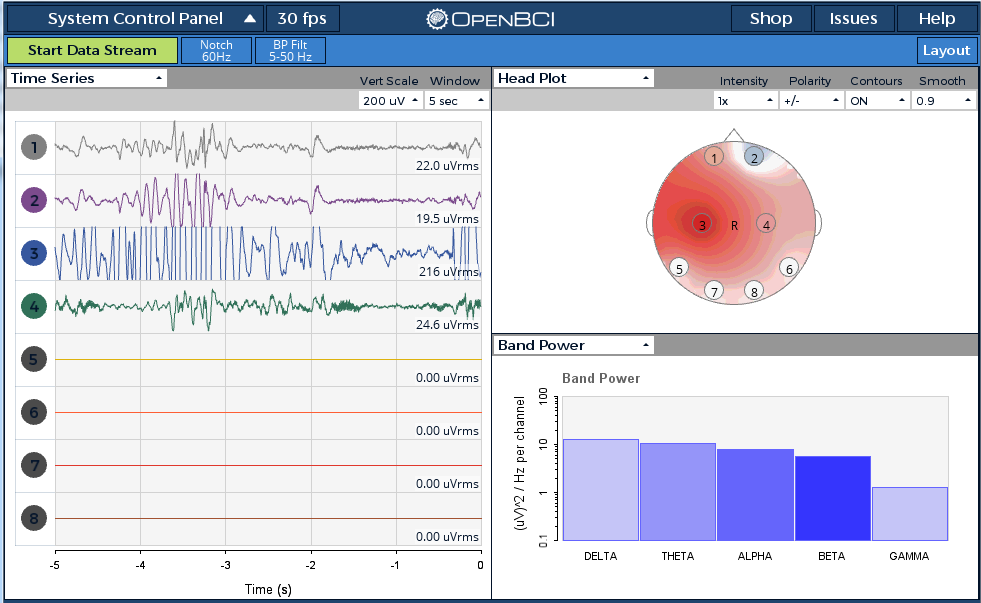Figure 57: Time domain raw EEG signal (4 channel), head plot and band power (bandpass filtered at 5-50 Hz and Notch filtered at 60 Hz). The UlTRACORTEX MARK IV headware and OPENBCI board is mounted on the subject and recording is done as shown in figure 58. Temporal cues during experiment are noted down by trained personal handling the equipment. EEG data are collected from 4 channels, FP1, FP2, F3, and F4 and digitized at a frequency of 250 Hz. Once EEG data are stored to a database with time-stamps for onset of temporal cues the next step is preprocessing. EEG signals stored by OPENBCI are amplified with a slowly moving DC “offset” which can go both positive and negative. To get rid of this, the collected EEG signal must first subject to millivolt DC offset using a high-pass filter at 0.5 Hz. A bandpass filter of 0-45 Hertz is applied to remove unwanted noise artifacts. Next the 60 Hz powerline noise is extinguished via band-stop filters and finally to avoid low/high frequency noise the EEG signals are band pass filtered between 0.1 and 60Hz. Then the FFT is taken and spectrum analysis are done to understand the power distribution of signals and to find out if there is any abnormality in frequency bands. After preprocessing EEG data is divided into two classes as follows: Class I included EEG data from eight experimental subjects recorded during their eyes-open relaxed (EO) stage; class II included EEG data recorded during their hyper arousal stage from the same eight subjects. As mentioned each subject completed the pre-intervention eyes open stage and hyperarousal intervention within a specified period. Hence, these EEG recordings are time stamped for the onset of cues and continuously for 3 minutes. Initial 30 sec and final 30 sec of the recording are avoided to clear of noise and artifacts and remaining 2 minutes recording is used feature extraction in both classes. This counts for 30000 samples per class for a single channel and data classification is done using features extracted from right prefrontal (FP2) which is consistent in all subjects. To maintain uniformity among the data since, multiple hyperarousal are common during meditation, in correlation with the physiological measurements first 10000 samples (from the extracted 30000 samples) covering the first hyperarousal are used for feature extraction. Each subject’s EEG recording are segmented into samples of 250 each and each EEG segment is considered as an observation; thus producing 40 observations per subject. Figure 58: Demo presentation of EEG headset and OPENBCI equipment connected to a person However, for a few subject’s data is not retrieved either due to large amount of noise or patients discomfort wearing the equipment. Thus, out of 8 subjects 6 subject’s data were able to use for pattern recognition and classification study. Totally, we observed 240 observations for class I from 6 subjects. To maintain balance between classes, class II data is also segmented according to same formula as a result the intervention data also included 240 observations. DWT employed on each observation verified how the time-frequency features varies for hyperarousal patterns when compared to the baseline pattern. 5.2.2.2 Hyperarousal Pattern Recognition The results are from six classifiers on the EEG data obtained from six subjects during soul retrieval experiment. Table 14 shows the comprehensive results for classification experiments on EEG data of 6 subjects, while table 15 displays the mean and standard deviation of the test accuracy of all classifiers involved in the study. Figure 61 displays the values of area under ROC curve for three experiments.

		Test

Subject Model Train Accuracy Accuracy Sensitivity Specificity Precision AUC S002 Decision Tree 100 79.16 73.33 88.88 57.89 0.81 KNN , N=2 80 70.83 80 55.55 70.58 SVM, Kernel = RBFN 70 62.5 46.6 88.8 46.6 MLP, HL=2, (10, 20) 100 87.5 93.33 77.7 66.66 K fold cross validation, k=5, HL=1, (10,) 100 96.25 LSTM, HL=2, (10, 20) 100 87.5 93.33 55.55 73.68

S001 Decision Tree 100 62.5 60 66.67 60 0.63 KNN , N=2 85 75 86.67 55.55 72.22 SVM, Kernel = RBFN 64 45.83 13.33 100 18.18 MLP, HL=2, (10, 20) 96.43 70.833 60 88.88 57.14 K fold cross validation, k=5, HL=1, (10,) 100 91.25 LSTM, HL=2, (10, 20) 75 70.83 53.33 100 47.05 0.76 S005 Decision Tree 100 70.83 53.33 100 47.05 KNN , N=2 82 66.67 60 77.77 56.25 SVM, Kernel = RBFN 62 41.66 6.66 100 10 MLP, HL=2, (10, 20) 100 70.833 60 88.88 52.94 K fold cross validation, k=5, HL=1, (10,) 100 88.75 LSTM, HL=2, (10, 20) 83 69.12 63.33 54.44 66.66

S008 Decision Tree 100 75 73.33 77.77 61.11 0.83 KNN , N=2 100 79.16 86.66 66.66 68.42 SVM, Kernel = RBFN 62 41.66 13.33 88.88 20 MLP, HL=2, (10, 20) 98 79.16 66.66 88.88 55.55 K fold cross validation, k=5, HL=1, (10,) 100 85 LSTM, HL=2, (10, 20) 98 80 80 77.77 63.15

S009 Decision Tree 100 91.67 100 77.77 68.18 0.85 KNN , N=2 85 75 86.66 55.55 72.22 SVM, Kernel = RBFN 66.66 33.33 6.67 77.77 12.5 MLP, HL=2, (10, 20) 100 87.5 80 100 57.14 K fold cross validation, k=5, HL=1, (10,) 100 90 LSTM, HL=2, (10, 20) 98.21 89.5 93.33 77.77 66.66

S006 Decision Tree 100 66.66 66.66 66.66 62.5 0.66 KNN , N=2 98 79.16 93.33 55.55 73.68 SVM, Kernel = RBFN 60 37.5 10 100 12 MLP, HL=2, (10, 20) 98.21 87.5 93.33 77.77 66.66 K fold cross validation, k=5, HL=1, (10,) 100 95 LSTM, HL=2, (10, 20) 100 79.16 80 77.77 63.15

Table 14: Classification performance of EEG data of six subjects in a two-class problem using time-frequency features.

	Test Accuracy	

System Decision Tree KNN SVM MLP K-Fold LSTM S001 62.5 75 45.83 70.83 91.25 70.83 S002 79.16 70.83 70.83 87.5 96.25 87.5 S005 70.83 66.67 41.66 70.833 88.75 69.12 S008 75 79.16 41.66 79.16 85 80 S009 91.67 75 33.33 87.5 90 89.5 S006 66.66 79.16 37.5 87.5 95 79.16 Mean 74.30 74.30 45.14 80.55 91.04 79.35 STD 9.45 4.44 12.13 7.48 3.78 7.61

Table 15: Mean and Standard Deviation of test accuracy of various classifier models used.

As shown in Table 14 for the subject 001, the performance of the k-fold cross validation of MLP, MLP and KNN classifiers showed 91.25,70.83 and 75 percentage of accuracy respectively. LSTM also shown equal performance as MLP. For subject 002, the best three accuracy performances are clocked by K-fold cross validation of MLP, MLP and equally by LSTM classifiers as 96.25,87.5and 87.5 respectively. For subject 005 the performance of k-fold cross validation of MLP, decision tree and MLP classifiers are 88.75,70.83 &70.83. For subject 008 the highest accuracy performances are given by k-fold cross validation of MLP, MLP and LSTM. Finally, in subject 009 the k-fold cross validation of MLP, LSTM and MLP records the highest accuracy performances. In addition, if we look at the conventional classifiers performance we can understand that most of their performance are in the range of 60’s with an exception to SVM classifier. The neural network-based classifiers fared better than the conventional statistical classifiers. If we look at other performance parameters, i.e., sensitivity, specificity and precision are also high. This impressive performance of artificial neural network-based classifiers reflects the effectiveness of neural networks in recognizing nonlinear dynamical patterns. These results also underlines the efficiency of time-frequency features for a classification task of complex EEG patterns. Subject wise classification accuracy for different systems are presented in Table 15. The mean and standard deviation of accuracies with Decision tree, KNN, SVM, MLP, k-fold cross validation of MLP and LSTM classifiers for six subjects are 74.30±9.45,74.30±4.44,45.14±4.13,80.55±7.48,91.04±3.78,79.35±7.61 respectively. From this we can understood that MLP with k- fold cross validation has best accuracy with a small variance followed by LSTM with decent performance and comparatively high variance next to MLP and decision tree and KNN, but SVM displayed inferior performance as an exception. Figure 61 represents area under ROC curve for MLP classifier, out of 6 subjects 4 of them has area under the curve around 0.8 and two of them around 0.6, this is a good performance and implies that MLP classifier is indeed a suitable classifier to separate complex brain patterns. All other parameters like accuracy, sensitivity, specificity and precision has shown decent performance. This gives more confidence to the results of the classifier.

Majority of classifiers registered an accuracy between 75% and 95%, which is a good performance with an exception of SVM. The normalization step during preprocessing helps the extracted features be more Gaussian improving classification accuracy. In addition, the results also confirm DWT’s ability to compactly represent EEG signals and extract unique representative features based on total and relative energy levels for different frequency bands. These results indicate that relative wavelet energy is an appropriate feature for identifying EEG patterns related to a complex mental state and classify it from another EEG pattern. The performance of nonlinear dynamical systems are better compared to EEG. The mean performance of each classifier for the 3 nonlinear dynamical systems using temporal-spectral features varies between excellent figures of 84.2 and 98.33, while that of EEG is between 45.14 and 91.04. The best accuracy achieved is also higher for nonlinear dynamical systems comparing to EEG signals. Even though EEG signals show similar nonlinear dynamics, EEG signals are meddled with noise, unwanted artifacts and EMG signals. On the other hand, nonlinear dynamical signals generated from equations are free from noise and external disturbances, this helps to improve the classifiers performance. Other results like sensitivity and specificity remains almost same for both EEG and nonlinear dynamical systems but the precision and AUC values of EEG signals are slightly higher than nonlinear dynamical counterparts. Results of previous pattern recognition and classification studies done on a publicly available cognitive EEG datasets are shown in table 16[101], where the performance are estimated using accuracy of classifier and best performance was achieved by DWT feature extraction method with SVM classifier for the multiplication task. Unlike this scenario, there aren’t any previous EEG signal classification and pattern recognition study done on the EEG dataset during soul retrieval process. Hence, a direct comparison with previous results on same dataset is not possible. So, comparison are done with dataset that are obtained from subjects having similar mental state during an experiment. Emotional stress pattern recognition from EEG signal has striking similarity with the traumatic memory retrieval and intervention process[23]. In [23] author reported results for classification of a two-class problem for 15 subjects, i.e., calm/neutral EEG patterns during relaxed mental state and negative excited EEG patterns during emotional stressed mental state are classified using an Elman Neural network and achieved a classification accuracy of 79.2 percentage. Another study done by Chanel et. al., tried to classify between calm vs negatively excited vs positively excited stage using linear classifiers LDA and SVM and achieved a three class classification accuracy of 67 percentage and a two class classification accuracy of 79 percentage[24]. An emotional stress detection system from EEG and other physiological signals designed by Khalizadeh et. al., used nonlinear features for classification using Elman ANN classifier with cross validation achieved an accuracy of 80 percentage for a two class classification task[25]. Comparison of the proposed approach with previous works on similar area is shown in table 17.

Study Classes Feature Extraction Methods Classifier Test Accuracy% Previous study[22] Calm vs Negative Excited Linear features- DWT, Nonlinear features- Correlation Dim, Fractal Dimension Elman Neural Network(5 fold cross-validation) 79.2 Previous study[23] Calm vs Excited Short Time Fourier Transform, sliding window of 512 samples, and 50% overlap LDA and SVM classifier 79 Previous study[24] Classify emotions into two main areas around valence arousal space Nonlinear features- Fractal dimension, Correlation Dimension, Approximate entropy Elman Neural Network(5 fold cross-validation) 80.1 Present study Calm vs Focused Guided Imagery Linear features- DWT+(Feature normalization) MLP, HL=2, (10, 20)(5 fold cross validation) 90.25

Table 17: Performance comparison between proposed approach and previous works on similar area. Compared to previous studies current study uses less complex feature extraction model and an advanced classifier, also the proposed feature extraction and optimization appear to have yielded a more efficient and reliable solution. The proposed pattern recognition scheme, as demonstrated in the present study, yielded higher accuracy rates with MLP with cross validation and LSTM, indicating superior discriminatory performances when assessing complex emotional tasks. 5.3 Ethical Considerations An application for EEG data collection was made to the University of Regina Ethics board and subsequently approved. All participants had signed the informed consent form before starting the experiment. All possible precautions were taken to maintain the confidentiality. All transcribed information was anonymized by removing any identifying information such as subject’s names, places, and regions.

5.4 Summary The goal of mental task classification and pattern recognition is to understand human brain functions. The study of pattern recognition and associate the patterns with a particular mental state can help identifying certain medical conditions and responding swiftly. Feature extraction is an important step for pattern recognition task and various techniques like linear and nonlinear dynamic features were successfully used for feature extraction and classification of EEG signals [23]. Since, EEG signals are time series signals two types of linear features, temporal- spectral as well as spatial features can depict the properties of the signal. Hence, it is important to verify the capability of temporal features and temporal-spectral features for pattern recognition tasks of nonlinear dynamical signals. In this chapter a new pattern recognition model based on statistical feature extraction method is proposed. At first, we study performance of proposed model on different classes of synthetically generated nonlinear dynamical signals. Performance of both temporal and temporal-spectral features are evaluated on the Lorenz, Chen’s and Rossler’s dataset using several classifiers. The overall classification performance of nonlinear dynamical systems with temporal-spectral features was found higher than of just temporal features. The performance of nonlinear dynamical system classification was compared with previous studies and found to be producing better results in terms of accuracy and the amount of features used. The performance of temporal-spectral feature-based classifiers in EEG pattern recognition is studied. The mentally aroused state during a holistic spiritual healing process known as hyperarousal is introduced in the work and EEG dataset during this mental state and baseline-relaxed mental state are also collected from PTSD subjects. A variety of machine learning based classifiers including Decision Tree, SVM, KNN, MLP, K fold MLP and LSTM are tasked of recognizing the hyperarousal patterns and classify it from the baseline pattern. The results show superior performance of proposed model for a two class pattern recognition when compared to the previous pattern recognition research efforts for EEG signals with similar mental state.