ClinicalBERT: Using Deep Learning Transformer Model to Predict Hospital Readmission

Before we begin, let me point you to my GitHub repo [or Jupyter Notebook] containing all the code used in this guide. Feel free to use the code to follow along with the guide. You can use this google link to download the pretrained ClinicalBERT model along with the readmission task fine-tuned model weights.

If you came here from my earlier work Predicting Hospital Readmission using NLP, this deep learning work won’t serve as a direct comparison for the AUROC metric because my approach is completely different in this paper. The more I dug into it, the more I discovered that the most beneficial application for clinicians is to be able to use these predictions to make adjustments while a patient is still in the hospital in order for Doctors to intervene and prevent them from being readmitted in the future. Therefore instead of using discharge summaries (written after a patient’s stay is over) it’s best to just feed in the early notes into the model that were gathered from within 2–3days of a patients stay.

My results for predicting readmission using only the first few days of notes in the intensive care unit (not discharge summaries) are:

• For 2days AUROC=0.748 and for 3days AUROC=0.758.

• For 2days RP80=38.69% and for 3days RP80=38.02%.

See the bottom of this article for full details.

I recently read this great paper “ClinicalBert: Modeling Clinical Notes and Predicting Hospital Readmission” by Huang et al (Paper & GitHub).

They develop ClinicalBert by applying BERT (bidirectional encoder representations from transformers) to clinical notes.

I wanted to dissect the work and expound upon the deep learning concepts. My work will serve as a detailed annotation (along with my own code changes) and interpretation of the contents of this academic paper. I will also create visualizations to enhance explanations. And I converted it to a convenient Jupyter Notebook format.

1. I am only working with early clinical notes (first 24–48 hrs and 48–72 hrs) because although discharge summaries have predictive power for readmission, “discharge summaries might be written after a patient has left the hospital. Therefore, discharge summaries are not actionable since doctors cannot intervene when a patient has left the hospital. Models that dynamically predict readmission in the early stages of a patient’s admission are relevant to clinicians…a maximum of the first 48 or 72 hours of a patient’s notes are concatenated. These concatenated notes are used to predict readmission.”pg 12. The ClinicalBERT model can predict readmission dynamically. Making a prediction using a discharge summary at the end of a stay means that there are fewer opportunities to reduce the chance of readmission. To build a clinically-relevant model, we define a task for predicting readmission at any timepoint since a patient was admitted.

2. My code is presented in a Jupyter Notebook rather than .py files.

3. It’s important to note that my code differs from Huang’s because I migrated to using HuggingFace’s new transformer module instead of the formerly known as pytorch_pretrained_bert that the author used.

4. I do not conduct pre-training the ClinicalBERT because the author already performed pre-training on Clinical words and the model’s weights are already available here.

BERT (Bidirectional Encoder Representations from Transformers) is a recent model published in Oct 2018 by researchers at Google AI Language. It has caused a stir in the Machine Learning community by presenting state-of-the-art results in a wide variety of NLP tasks, including Question Answering (SQuAD v1.1), Natural Language Inference (MNLI), and others.

ClinicalBERT is a Bidirectional Transformer.

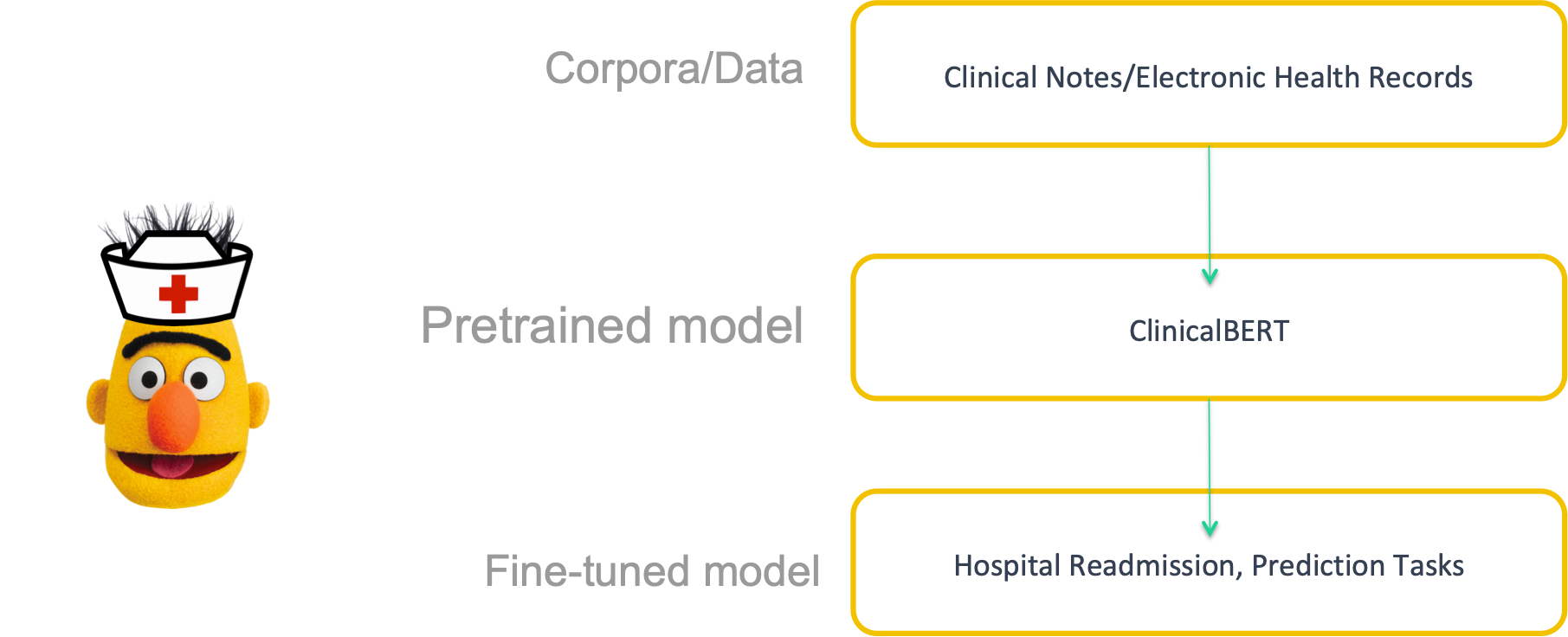
ClinicalBERT is a modified BERT model: Specifically, the representations are learned using medical notes and further processed for downstream clinical tasks.

ClinicalBERT is pretrained on patient clinical notes/EHR and then can be used for downstream predictive tasks.

The diagram below illustrates how care providers add notes to an electronic health record during a patient’s admission, and the model dynamically updates the patient’s risk of being readmitted within a 30-day window.

Every day, more data gets added to an EHR. Notes like Radiology, Nursing, ECG, Physician, Discharge summary, Echo, Respiratory, Nutrition, General, Rehab Services, Social Work, Case Management, Pharmacy and Consult.

Before the author even evaluated ClinicalBERT’s performance as a model of readmission, his initial experiment showed that the original BERT suffered in performance on the masked language modeling task on the MIMIC-III data as well as the next sentence prediction tasks. This proves the need develop models tailored to clinical data such as ClinicalBERT!

Medicine suffers from alarm fatigue. This means useful classification rules for medicine need to have high precision (positive predictive value).

The quality of learned representations of text depends on the text the model was trained on. Regular BERT is pretrained on BooksCorpus and Wikipedia. However, these two datasets are distinct from clinical notes. Clinical notes have jargon, abbreviations and different syntax and grammar than common language in books or encyclopedias. ClinicalBERT is trained on clinical notes/Electronic Health Records (EHR).

Clinical notes require capturing interactions between distant words and ClinicalBert captures qualitative relationships among clinical concepts in a database of medical terms.

Compared to the popular word2vec model, ClinicalBert more accurately captures clinical word similarity.

[Source]

Just like BERT, Clinical BERT is a trained Transformer Encoder stack.

Here’s a quick refresher on the basics of how BERT works.

[Source]

BERT base has 12 encoder layers.

In my code I am using BERT base uncased.

[Source]

Pretrained BERT has a max of 512 input tokens (position embeddings). The output would be a vector for each input token. Each vector is made up of 768 float numbers (hidden units).

ClinicalBERT outperforms BERT on two unsupervised language modeling tasks evaluated on a large corpus of clinical text. In masked language modeling (where you mask 15% of the input tokens and using the model to predict the next tokens) and next-sentence prediction tasks ClinicalBERT outperforms BERT by 30 points and 18.75 points respectively.

Source: https://arxiv.org/abs/1904.05342

ClinicalBERT can be readily adapted to downstream clinical tasks e.g. Predicting 30-Day Readmission.

In this tutorial, we will use ClinicalBERT to train a readmission classifier. Specifically, I will take the pre-trained ClinicalBERT model, add an untrained layer of neurons on the end, and train the new model.

You might be wondering why we should do fine-tuning rather than train a specific deep learning model (BiLSTM, Word2Vec, etc.) that is well suited for the specific NLP task you need?

• Quicker Development: The pre-trained ClinicalBERT model weights already encode a lot of information about our language. As a result, it takes much less time to train our fine-tuned model — it is as if we have already trained the bottom layers of our network extensively and only need to gently tune them while using their output as features for our classification task. For example in the original BERT paper the authors recommend only 2–4 epochs of training for fine-tuning BERT on a specific NLP task, compared to the hundreds of GPU hours needed to train the original BERT model or a LSTM from scratch!

• Less Data: Because of the pretrained weights this method allows us to fine-tune our task on a much smaller dataset than would be required in a model that is built from scratch. A major drawback of NLP models built from scratch is that we often need a prohibitively large dataset in order to train our network to reasonable accuracy, meaning a lot of time and energy had to be put into dataset creation. By fine-tuning BERT, we are now able to get away with training a model to good performance on a much smaller amount of training data.

• Better Results: Fine-tuning is shown to achieve state of the art results with minimal task-specific adjustments for a wide variety of tasks: classification, language inference, semantic similarity, question answering, etc. Rather than implementing custom and sometimes-obscure architectures shown to work well on a specific task, fine-tuning is shown to be a better (or at least equal) alternative.

ClinicalBert is fine-tuned on a task specific to clinical data: readmission prediction.

The model is fed a patient’s clinical notes, and the patient’s risk of readmission within a 30-day window is predicted using a linear layer applied to the classification representation, hcls, learned by ClinicalBert.

The model parameters are fine-tuned to maximize the log-likelihood of this binary classifier.

Here is the probability of readmission formula:

P (readmit = 1 | hcls) = σ(W hcls)

• readmit is a binary indicator of readmission (0 or 1).

• σ is the sigmoid function

• hcls is a linear layer operating on the final representation for the CLS token. In other words hcls is the output of the model associated with the classification token.

• W is a parameter matrix

Before starting you must create the following directories and files:

Run this command to install the HuggingFace transformer module:

conda install -c conda-forge transformers

I used the MIMIC-III dataset that they host in the cloud in an S3 bucket. I found it was easiest to simply add my AWS account number to my MIMIC-III account and use this link s3://mimic-iii-physionet to pull the ADMISSIONS and NOTEEVENTS table into my Notebook.

ClinicalBert requires minimal preprocessing:

1. First, words are converted to lowercase

2. Line breaks are removed

3. Carriage returns are removed

4. De-identified the personally identifiable info inside the brackets

5. Remove special characters like ==, −−

6. The SpaCy sentence segmentation package is used to segment each note (Honnibal and Montani, 2017).

Since clinical notes don’t follow rigid standard language grammar, we find rule-based segmentation has better results than dependency parsing-based segmentation. Various segmentation signs that misguide rule-based segmentators are removed or replaced.

• For example 1.2 would be removed.

• M.D., dr. would be replaced with with MD, Dr

• Clinical notes can include various lab results and medications that also contain numerous rule-based separators, such as 20mg, p.o., q.d.. (where q.d. means one a day and q.o. means to take by mouth.

• To address this, segmentations that have less than 20 words are fused into the previous segmentation so that they are not singled out as different sentences.

I used a Notebook in AWS Sagemaker and trained on a single p2.xlarge K80 GPU (in SageMaker choose the ml.p2.xlarge). You will have to request a limit increase from AWS support before you can use a GPU. It is a manual request that’s ultimately granted by a human being and could take several hours or 1-day.

Create a new Notebook in SageMaker. Then open a new Terminal (see picture below):

Copy/paste and run the script below to cd into the SageMaker directory and create the necessary folders and files:

cd SageMaker/

mkdir -p ./data/discharge

mkdir -p ./data/3days

mkdir -p ./data/2days

touch ./data/discharge/train.csv

touch ./data/discharge/val.csv

touch ./data/discharge/test.csv

touch ./data/3days/train.csv

touch ./data/3days/val.csv

touch ./data/3days/test.csv

touch ./data/2days/test.csv

Upload your Notebook that you’ve been working in on your local computer.

When creating an IAM role, choose the Any S3 bucket option.

Create a /pickle directory and upload the 3 pickled files: df_discharge.pkl, df_less_2.pkl and df_less_3.pkl. This may take a few minutes because the files are 398MB, 517MB, and 733MB respectively.

Then upload the modeling_readmission.py and file_utils.py files into the Jupyter home directory.

Then upload the model directory to the Jupyter home directory. You can create the directory structure using the following command: mkdir -p ./model/early_readmission. Then you can upload the 2 files pytorch_model.bin and bert_config.json into that folder. This may take a few minutes because pytorch_mode.bin is 438MB.

Ultimately your Jupyter directory structure should look like this:

Note that the result_early folder will be created by the code (not you).

Now you can run the entire notebook.

Running the entire notebook took about 8 minutes on a K80 GPU.

If you’d like to save all of the files (including output) to your local computer run this line in your Jupyter Notebook: !zip -r -X ClinicalBERT3_results.zip './' then you can download it manually from your Notebook.

There’s quite a bit of code so let’s walk through the important bits. I’ll skip a lot of the preprocessing parts like cleaning, splitting training/val/test sets and subsampling that I already covered in-depth here.

# to get 318 words chunks for readmission tasks
    df_len = len(df_less_n)
    want = pd.DataFrame({'ID': [], 'TEXT': [], 'Label': []})
    for i in tqdm(range(df_len)):
        x = df_less_n.TEXT.iloc[i].split()
        n = int(len(x) / 318)
        for j in range(n):
            want = want.append({'TEXT': ' '.join(x[j * 318:(j + 1) * 318]), 'Label': df_less_n.OUTPUT_LABEL.iloc[i],
                                'ID': df_less_n.HADM_ID.iloc[i]}, ignore_index=True)
        if len(x) % 318 > 10:
            want = want.append({'TEXT': ' '.join(x[-(len(x) % 318):]), 'Label': df_less_n.OUTPUT_LABEL.iloc[i],
                                'ID': df_less_n.HADM_ID.iloc[i]}, ignore_index=True)

A patient will usually have a lot of different notes, however, the ClinicalBert model has a fixed maximum length of input sequence. We split notes into subsequences (each subsequence is the maximum length supported by the model), and define how ClinicalBert makes predictions on long sequences by binning the predictions on each subsequence.

You might be wondering why we split into 318 word pieces? Because with BERT there’s a 512 maximum sequence number of sub word unit tokens (average ~318 words). In other words, BERT uses sub word units (WordPieces) instead of the entire word as the input unit. So instead of “I am having lunch” as 4 individual words, conceptually, it might do something like “I am hav ing lun ch”.

If you’d like to know more about it this paper was originally written to tackle the “out of vocab” problem but it turns out to have stronger predictive values.

The probability of readmission for a patient is computed as follows. Assume the patient’s clinical notes are represented as n subsequences and fed to the model separately; the model outputs a probability for each subsequence. The probability of readmission is computed using the probabilities output for each of these subsequences:

Equation for Probability of Readmission where c is a scaling factor that controls the amount of influence of the number of subsequences n, and hpatient is the implicit representation ClinicalBert computes from the entirety of a patient’s notes. Pnmax is the maximum of probability of readmission across the n subsequences, and Pnmean is the mean of the probability of readmission across the n subsequences a patient’s notes have been split into.

Huang finds that computing readmission probability using the equation above 11consistently outperforms predictions on each subsequence individually by 3-8%. This is because:

1. Some subsequences, n, (such as tokens corresponding to progress reports) do NOT contain information about readmission, whereas others do. The risk of readmission should be computed using subsequences that correlate with readmission risk, and the effect of unimportant subsequences should be minimized. This is accomplished by using the maximum probability over subsequences (Pnmax).

2. Also noisy subsequences mislead the model and decrease performance. So they also include the average probability of readmission across subsequences (Pnmean). This leads to a trade-off between the mean and maximum probabilities of readmission.

3. If there are a large number of subsequences for a patient with many clinical notes, there is a higher probability of having a noisy maximum probability of readmission. This means longer sequences may need to have a larger weight on the mean prediction. We include this weight as the n/c scaling factor, with c adjusting for patients with many clinical notes. Empirically, Huang found that c=2 performs best on validation data.

The formula can be found in the vote_score function in the temp variable Remember that the 2 is from c=2:

def vote_score(df, score, readmission_mode, output_dir):
    df['pred_score'] = score
    df_sort = df.sort_values(by=['ID'])
    #score
    **temp = (df_sort.groupby(['ID'])['pred_score'].agg(max)+df_sort.groupby(['ID'])['pred_score'].agg(sum)/2)/(1+df_sort.groupby(['ID'])['pred_score'].agg(len)/2)**
    x = df_sort.groupby(['ID'])['Label'].agg(np.min).values
    df_out = pd.DataFrame({'logits': temp.values, 'ID': x})

fpr, tpr, thresholds = roc_curve(x, temp.values)
    auc_score = auc(fpr, tpr)

plt.figure(1)
    plt.plot([0, 1], [0, 1], 'k--')
    plt.plot(fpr, tpr, label='Val (area = {:.3f})'.format(auc_score))
    plt.xlabel('False positive rate')
    plt.ylabel('True positive rate')
    plt.title('ROC curve')
    plt.legend(loc='best')
    plt.show()
    string = 'auroc_clinicalbert_'+readmission_mode+'.png'
    plt.savefig(os.path.join(output_dir, string))

return fpr, tpr, df_out

For validation 10% of the data is held out, for testing 10% of the data is held out, then 5-fold cross-validation is conducted.

Each model is evaluated using three metrics:

1. Area under the ROC curve (AUROC)

2. Area under the precision-recall curve (AUPRC)

3. Recall at precision of 80% (RP80): For the readmission task, false positives are important. To minimize the number of false positives and thus minimize the risk of alarm fatigue, we set the precision to 80%. In other words we set a 20% false positive rate out of the predicted positive class and use the corresponding threshold to calculate recall. This leads to a clinically-relevant metric that enables us to build models that control the false positive rate.

Here is the code: https://gist.github.com/nwams/faef6411b342cf163d6c8fb6267433f9#file-clinicalbert-evaluation-py

Here are the results output from Predicting Readmission on the Early Notes:

I recommend reading Jason Brownlee’s article.

• Precision is a ratio of the number of true positives divided by the sum of the true positives and false positives. It describes how good a model is at predicting the positive class. It is also referred to as the positive predictive value.

• Recall, a.k.a. sensitivity, is calculated as the ratio of the number of true positives divided by the sum of the true positives and the false negatives.

It’s important to look at both precision and recall in cases where there is an imbalance in the observations between the two classes. Specifically, when there are many examples of no event (class 0) and only a few examples of an event (class 1). Because usually the large number of class 0 examples means we are less interested in the skill of the model at predicting class 0 correctly, e.g. high true negatives.

The important thing to note in the calculation of precision and recall is that the calculations do not make use of the true negatives. It is only concerned with the correct prediction of the minority class, class 1.

The recommendations are:

• ROC curves should be used when there are roughly equal numbers of observations for each class.

• Precision-Recall curves should be used when there is a moderate to large class imbalance.

Why? Because ROC curves present an overly optimistic picture of the model on datasets with a class imbalance. It’s optimistic because of the use of true negatives in the False Positive rate in the ROC Curve; however remember that the False Positive rate is carefully avoided in the Precision-Recall.

For 2days AUROC=0.748 and for 3days AUROC=0.758.

For 2days RP80=38.69% and for 3days RP80=38.02%.

Based on experimentation, ClinicalBert outperforms results from Bag-of-Words and BILSTM baselines. Unfortunately, I didn’t find any other papers/studies that focused solely on early notes, which could’ve been a nice additional comparison point. Nevertheless, the table below shows that the outperformance can be “up to” the following:

I’d like to emphasize that this only gives the upper bound on the delta of the metrics. The green arrows just indicates that ClinicalBERT has improved performance compared to Bag of Words and BILSTM in all of these metrics for both the 2-days and 3-day results.

Since we balanced the data I’ll focus on reporting the AUROC curve as the most appropriate metric instead of the AUPRC.

I’ll also focus on reporting the Recall at 80% Precision metric due to the fact that it is clinically relevant (remember that alarm fatigue is a real problem in healthcare that we are intentionally trying to avoid/reduce).

ClinicalBERT has more confidence compared to the other models. And at a fixed rate of false alarms, ClinicalBert recalls more patients that have been readmitted.

• Up to 9.5% AUROC compared to Bag-of-Words and up to 6.5% AUROC when compared to BILSTM.

• Up to 20.7% RP80 compared to Bag-of-words and up to 19.4% RP80 when compared to BILSTM.

• Up to 9.8% AUROC compared to Bag-of-Words and up to 9.6% AUROC when compared to BILSTM.

• Up to 26.2% RP80 compared to Bag-of-words and up to 20.9% RP80 when compared to BILSTM.

The code I used for creating the self-attention map in this section is here.

It’s very difficult for a human to understand why a neural network made a certain prediction, and what parts of the input data did the model find most informative. Therefore Doctors may not trust output from a data-driven method.

Well, visualizing the self-attention mechanism is a way to solve that problem because it allows you to see the terms correlated with predictions of hospital readmission.

You might already be familiar with the popular “Attention is All You Need” paper that was submitted at the 2017 arXiv by the Google machine translation team. If not, check out this animation that explains attention. More intuitively, we can think “self-attention” as the sentence will look at itself to determine how to represent each token.

As the model processes each word (each position in the input sequence), self attention allows it to look at other positions in the input sequence for clues that can help lead to a better encoding for this word.

— The Illustrated Transformer by Jay Alammar

For every clinical note input to ClinicalBert, each self-attention mechanism computes a distribution over every term in a sentence, given a query. The self-attention equation is:

Where q is query vector, K is the key vector, d is the dimensionality of the queries and keys.

Intuitively, we can think of it like this: the query, q, represents what kind of information we are looking for, and the key, K, represent the relevance to the query.

A high attention weight between a query and key token means the interaction between these tokens is predictive of readmission. In the ClinicalBert encoder, there are 144 heads (which is 12 multi-head attention mechanisms for each of the 12 encoder layers). There will be diversity in the different heads, which is what we should expect because different heads learn different relations between word pairs. Although each head receives the same input embedding, through random initialization, each learns different focuses [img].

The self-attention map below is just one of the self-attention heads in ClinicalBERT — it reveals which terms in clinical notes are predictive of patient readmission. The sentence he has experienced acute on chronic diastolic heart failure in the setting of volume overload due to his sepsis . is used as input that is fed into the model. This sentence is representative of a clinical note found in MIMIC-III. The SelfAttention equation is used to compute a distribution over tokens in this sentence, where every query token, q, is also a token in the same input sentence.

ClinicalBERT Self-Attention Map. The darker colors stand for greater weights.

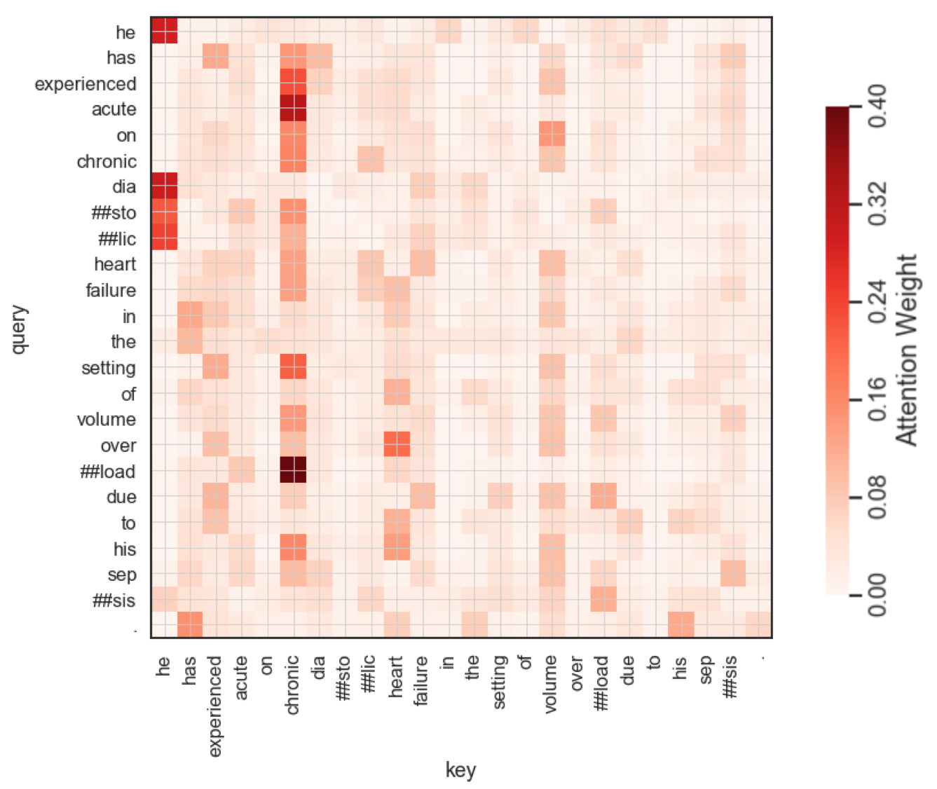
Notice that the self-attention map shows a higher attention weight between the the word chronic and acute…or chronic and ###load .

Intuitively, the presence of the token associated with the word “chronic” is a predictor of readmission.

Remember though, there are 12 heads at each layer (144 total heads for this model). And each head is looking at different things. So looking at each head’s attention graph separately will give you an understanding of how the model makes predictions — but it won’t make it super easy to interpret the entire system as a “one-stop shop”. Instead, you could do some aggregation (summing up or averaging all the attention head’s weights).

So if you’re a clinician looking for a “one-stop shop” understanding of the help with interpretation exBERT is an interactive software tool that provides insights into the meaning of the contextual representations by matching a human-specified input to similar contexts in a large annotated dataset. By aggregating the annotations of the matching similar contexts, exBERT helps intuitively explain what each attention-head has learned [Paper]. Although this was created for BERT, this type of tool could also be adapted to ClinicalBERT as well!

As an aside, if you’re interested in learning more about the heads, and self-attention weights as it pertains to several BERT NLP tasks, I highly, highly, recommend this academic paper, Revealing the Dark Secrets of BERT — it does a great job at dissecting and investigating the self-attention mechanism behind BERT-based architectures.

@article{clinicalbert,
author = {Kexin Huang and Jaan Altosaar and Rajesh Ranganath},
title = {ClinicalBERT: Modeling Clinical Notes and Predicting Hospital Readmission},
year = {2019},
journal = {arXiv:1904.05342},
}

MIMIC-III, a freely accessible critical care database. Johnson AEW, Pollard TJ, Shen L, Lehman L, Feng M, Ghassemi M, Moody B, Szolovits P, Celi LA, and Mark RG. Scientific Data (2016). DOI: 10.1038/sdata.2016.35. Available at: http://www.nature.com/articles/sdata201635