This app will allow you to build & apply calibrations for the Tracer & Artax series of XRF devices. It (currently) works with .csv files produced from S1PXRF, PDZ versions 24 and 25, .spx files, Elio spectra (.spt), .mca files, and .csv files of net counts produced from Artax (7.4 or later).

It is based on the Lucas-Tooth and Price (1961) algorithm¹, though I have added modifications to make it more robust (it's really hard to get a validation plot slope that isn't 1). The algorithm goes like this:

C_i = r₀ + I_i[r_i + Σ(r_inI_n]

Where C_i represents the concentration of element, r₀ is the intercept/empirical constant for element i, r_i is the slope/empirical coefficient for intensity of element i, r_in is the slope/empirical constant for effect of element n on element i, I _i is the net intensity of element i, and I_n is the net intensity of element n. This equation is based on a simple linear model,

y = mx + b

In which y is C_i, b is r₀, m is r_i, and I_i is x (eg. C_i = r_iI_i + r₀). The additional variables present in the Lukas-Tooth equation indicate a slope correction for an element which influences the fluorescence of the element to be analyzed (subscript i represents the element being analyzed, subscript n represents the influencing element).

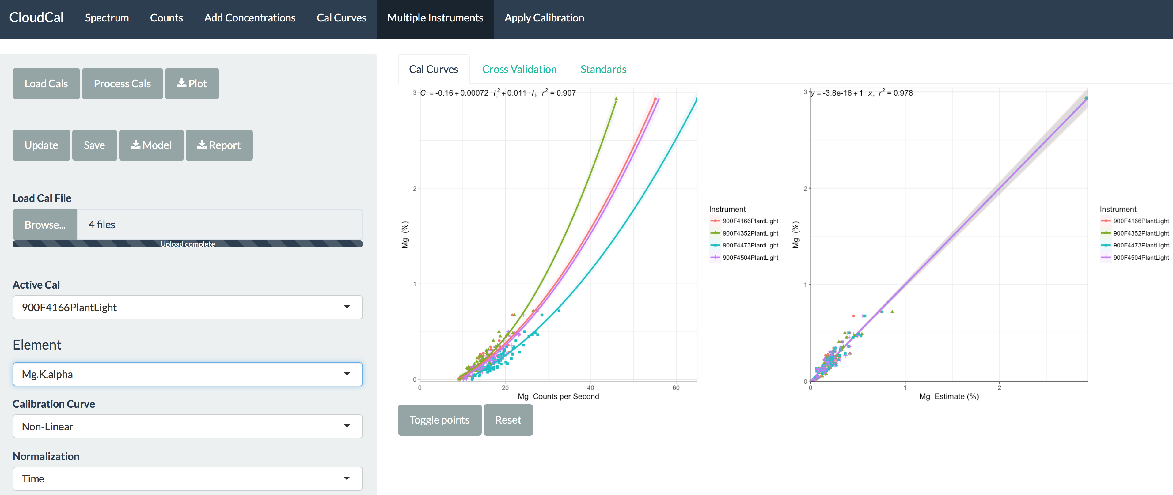
The algorithm is simply a way to a) estimate concentrations from the x-ray spectrum, b) account for variation from the spectrum itself, and c) make results from instruments comparable to one another reliably². That said, you do not have to use a Lucas-Tooth model to calibrate - in the app you can also choose linear/nonlinear models.

First, you will need to download a copy of R appropriate for your computer (Mac, Windows, or Linux):

https://www.r-project.org/

Next, you will need to install a package called 'shiny' to run it locally. You can do so by pasting this line into the R consul when you launch it:

install.packages(c("Rcpp", "shiny"))

It will ask you to choose a download mirror (you can choose anyone, the result is the same). Then, to run the software:

shiny::runGitHub("leedrake5/CloudCal")

The first time it runs, it may take some time to download the supporting software. After that, you should be good to go. If you'd like to download a copy and run it offline, you can instead download it from GitHub (https://github.com/leedrake5/CloudCal) and then run it locally:

shiny::runApp("your/computer/directory/CloudCal")

Currently, the data operates with .csv files exported from either S1PXRF or Artax, PDZ versions 24 and 25 (expiremental), and all three data formats associated with XG Lab's Elio (.spt, .spx, and .mca).

To export from S1PXRF, go to Setup -> Group Conversion. Then choose a directory with PDZ files and select 'CSV' as the output. I'd also choose 'Replace duration with live time' to make sure dead time in the spectra is not a problem. This will produce the CSV files that you need to run in the app.

For Artax, follow all the same steps you know (if you don't know, visit www.xrf.guru). Instead of going to Export -> All Results to Excel, go to Export -> All Results. This will create CSV files that can be read into the app as well.

Quick note - with the new Tracer 5i, Bruker has changed the format of PDZ files. That means data taken with the 5i is not compatible with the IISD/IVSD/IIV+, and vice-versa. Good news is that the most recent copy of Artax (8+) can handle both, but older copies won't. You'll need to convert from v25 (5i version) to v24 (Classic Tracer) to bring them in to S1PXRF - you can do this with CalToolkit or any other software Bruker provides. You can upload the PDZ files directly, but there may be problems - it doesn't work perfectly yet.

This filetype is an open-source way of holding all the data in a file. If you want to see what it looks like, enter the following code into R:

str(readRDS("location/of/your/file.quant"))

The result will be a lot of information, but here is the basic layout:

>$FileType (this defines the kind of csv you upload)
>$Units (these are the units you entered into the app - one type for everything) 
>$Spectra (this includes all the spectra of the csv files used to make the cal)
>$Intensities (these are the intensities of the elements you choose in the 'Counts' tab)
>$Values (these are the intensity data you put into the app)
>$calList (this is the holder for all the element models defined by you) 
	>$Element this is all the data for one element
		>$CalTable (this has all the settings for the element)
			>$CalType (this is whether or not Lucas-Tooth is used)
			>$NormType (this is they type of normalization you used)
			>$Min (this is the minimum normalization energy you chose)
			>$Max (this is the maximum normalization energy you chose)
		>$Slope (these are the slope variables you choose if you make a Lucas-Tooth cal)
		>$Intercept (these are the intercept variables you choose if you make a Lucas-Tooth cal)
		>$StandardsUsed (this is a list of the standards you used for the regressions) 
		>$Model (this is the parameters of the model you chose) 

No reason not to - I started with the Tracer because it was the easiest to work with & the best for custom quantification. The app has since been expanded to include Artax, the Picofox, and the Elio. If you have other instruments you'd like to add, let me know and I can see if I can do it. It will be some time before I can look into it though. Keep in mind that the software would need a heavy lift from multiple folks to read binary files - these are the proprietary company files that have non-open source file types.

You can cite this Github page:

v3.0 Drake, B.L. 2018. CloudCal v3.0. GitHub. https://github.com/leedrake5/CloudCal. doi: 10.5281/zenodo.2596154

Kuhn, M. 2008. Building predictive models iin R using the caret package. Journal of Statsitical Software. Journal of Statistical Software 28(5): 1-26 Liaw, A., Wiener, M. 2002. Classification and Regression by randomForest. R News 2(3): 18--22 Lucas-Tooth, H.J., Price, B.J. 1961. A Mathematical Method for the Investigation of Interelement Effects in X-Ray Fluorescence Analysis Metallurgia 64: 149–152 Speakman, R.J., Shackley, M.S. 2013. Silo science and portable XRF in archaeology: a response to Frahm. Journal of Archaeological Science 40: 1435-1443 Venables, W. N., Ripley, B. D. 2002. Modern Applied Statistics with S. Fourth Edition. Springer, New York. ISBN 0-387-95457-0