This repository contains data and analyses from the ASSIP 24-months follow-up randomized controlled study.
We provide a short analysis script (survival.R) to replicate the main findings of our study using the original data (assip.RData). Results in our paper may slightly differ because these are based on twenty imputed dataset. Variable description and statistical output see below.
Gysin-Maillart A, Schwab S, Soravia LM, Megert M, & Michel K (2016). A Novel Brief Therapy for Patients Who Attempt Suicide: A 24-months follow-up randomized controlled study of the Attempted Suicide Short Intervention Program (ASSIP). PLoS Medicine 13(9):e1001968. 10.1371/journal.pmed.1001968.
Article in The Washington Post.
amb_sess_t1_6M	Number of outpatient sessions at time one (t1), including the last 6 months
bdisum2		BDI (Beck Depression Intventory) sum, after 6 months (t2)
bdisum3		BDI (Beck Depression Intventory) sum, after 12 months (t3)
bdisum4		BDI (Beck Depression Intventory) sum, after 18 months (t4)
bdisum5		BDI (Beck Depression Intventory) sum, after 24 months (t5)
BSS_T2		BSS (Beck Scale for Suicide Ideation) mean, after 6 months (t2)
BSS_T3		BSS (Beck Scale for Suicide Ideation) mean, after 12 months (t3)
BSS_T4		BSS (Beck Scale for Suicide Ideation) mean, after 18 months (t4)
BSS_T5		BSS (Beck Scale for Suicide Ideation) mean, after 24 months (t5)
ITT			Intention to treat
repeater_t2		repeated suicide attempts (patient), 1-6 months, dichotomous(0, minimum 1 suicide attempt)
repeater_t3		repeated suicide attempts (patient), 6-12 months, dichotomous(0, minimum 1 suicide attempt)
repeater_t4		repeated suicide attempts (patient), 12-18 months, dichotomous(0, minimum 1 suicide attempt)
repeater_t5		repeated suicide attempts (patient), 18-24 months, dichotomous(0, minimum 1 suicide attempt)
stat_days_t1	Inpatient days at baseline (6 months backward)
sum_stat_12months	Sum of inpatient days after 12 months
sum_stat_24months	Sum of outpatient days after 24 months
> fit = survfit(Surv(time, repeater) ~ group, type="kaplan-meier")
> summary(fit)
Call: survfit(formula = Surv(time, repeater) ~ group, type = "kaplan-meier")
65 observations deleted due to missingness
group=ASSIP & ASSIP Drop out
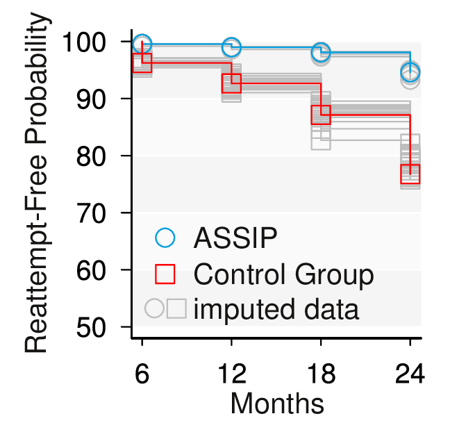
time n.risk n.event survival std.err lower 95% CI upper 95% CI
6 229 1 0.996 0.00436 0.987 1
12 170 1 0.990 0.00727 0.976 1
18 111 1 0.981 0.01143 0.959 1
24 56 2 0.946 0.02671 0.895 1
group=CG & CG Drop out
time n.risk n.event survival std.err lower 95% CI upper 95% CI
6 186 7 0.962 0.0140 0.935 0.990
12 134 5 0.926 0.0207 0.887 0.968
18 84 5 0.871 0.0308 0.813 0.934
24 42 5 0.768 0.0513 0.673 0.875
>
> # group difference (Mantel-Haenszel) ----
> survdiff(Surv(time, repeater) ~ group, rho=0)
Call:
survdiff(formula = Surv(time, repeater) ~ group, rho = 0)

n=415, 65 observations deleted due to missingness.

                               N Observed Expected (O-E)^2/E (O-E)^2/V
group=ASSIP & ASSIP Drop out 229        5     15.2      6.83      16.1
group=CG & CG Drop out       186       22     11.8      8.78      16.1

 Chisq= 16.1  on 1 degrees of freedom, p= 5.99e-05
For hazard ratio see exp(-coef) below
> # Cox hazard for discrete data ----
> hazard <- coxph(Surv(time, repeater) ~ group, ties="exact")
> summary(hazard)
Call:
coxph(formula = Surv(time, repeater) ~ group, ties = "exact")

  n= 415, number of events= 27
   (65 observations deleted due to missingness)

                        coef exp(coef) se(coef)     z Pr(>|z|)
groupCG & CG Drop out 1.7826    5.9451   0.5006 3.561 0.000369 ***
---
Signif. codes:  0 ‘***’ 0.001 ‘**’ 0.01 ‘*’ 0.05 ‘.’ 0.1 ‘ ’ 1

                      exp(coef) exp(-coef) lower .95 upper .95
groupCG & CG Drop out     5.945     0.1682     2.229     15.86

Rsquare= 0.04   (max possible= 0.421 )
Likelihood ratio test= 16.75  on 1 df,   p=4.268e-05
Wald test            = 12.68  on 1 df,   p=0.0003695
Score (logrank) test = 16.11  on 1 df,   p=5.992e-05
In the traditional survival analysis an event is generally associated with "death", and only one event is possible per subject (non-recurring events). However, recurring events relax this assumption and are also widely used in the literature, for example multiple relapses from remission for leukemia patients, repeated heart attacks, recurrence of bladder cancer tumors, or deteriorating episodes of visual acuity (Kleinbaum & Klein, 2005). Recurring analysis can be seen as repeated measures analysis, however one issue is that observations are not completely independent. Therefore, we also performed the analysis using non-recurring events.
E='Suizidversuch (mind. 1)'
time=rep(NA,120)
event=rep(NA,120)
for (i in 1:120) {
  f = c(mydata$repeater_t2[i]==E, mydata$repeater_t3[i]==E, mydata$repeater_t4[i]==E, mydata$repeater_t5[i]==E)
  if (sum(f, na.rm = T) > 0) { # time to event
	    time[i]=which(f)[1]*6; event[i]=1
  } else {  # censoring
	    c=tail(which(!f), n=1)
	    if (length(c) > 0) {time[i]=c*6; event[i]=0}
	    else {time[i]=0; event[i]=0}
  }
}
> fit = survfit(Surv(time, event) ~ mydata$ITT, type="kaplan-meier")
> summary(fit)
Call: survfit(formula = Surv(time, event) ~ mydata$ITT, type = "kaplan-meier")

    	        mydata$ITT=ASSIP & ASSIP Drop out
time n.risk n.event survival std.err lower 95% CI upper 95% CI
 6     59       1    0.983  0.0168        0.951        1.000
12     58       1    0.966  0.0236        0.921        1.000
18     54       1    0.948  0.0291        0.893        1.000
24     53       2    0.912  0.0374        0.842        0.989

    	        mydata$ITT=CG & CG Drop out
time n.risk n.event survival std.err lower 95% CI upper 95% CI
 6     53       7    0.868  0.0465        0.781        0.964
12     44       3    0.809  0.0545        0.709        0.923
18     37       4    0.721  0.0637        0.607        0.858
24     30       2    0.673  0.0680        0.552        0.821
> fit = survfit(Surv(time, event) ~ mydata$ITT, type="kaplan-meier")
> summary(fit)

Call:
survdiff(formula = Surv(time, event) ~ mydata$ITT, rho = 0)

                                   N Observed Expected (O-E)^2/E (O-E)^2/V
mydata$ITT=ASSIP & ASSIP Drop out 60        5    12.01      4.09      10.1
mydata$ITT=CG & CG Drop out       60       16     8.99      5.47      10.1

Chisq= 10.1  on 1 degrees of freedom, p= 0.00148
> hazard <- coxph(Surv(time, event) ~ mydata$ITT, ties="exact")
> summary(hazard)
Call:
coxph(formula = Surv(time, event) ~ mydata$ITT, ties = "exact")

n= 120, number of events= 21

                             coef exp(coef) se(coef)     z Pr(>|z|)
mydata$ITTCG & CG Drop out 1.5294    4.6156   0.5228 2.926  0.00344 **
---
Signif. codes:  0 ‘***’ 0.001 ‘**’ 0.01 ‘*’ 0.05 ‘.’ 0.1 ‘ ’ 1

                           exp(coef) exp(-coef) lower .95 upper .95
mydata$ITTCG & CG Drop out     4.616     0.2167     1.657     12.86

Rsquare= 0.082   (max possible= 0.71 )
Likelihood ratio test= 10.22  on 1 df,   p=0.001386
Wald test            = 8.56  on 1 df,   p=0.003436
Score (logrank) test = 10.11  on 1 df,   p=0.001478