Giter Club home page Giter Club logo

cellpylib's Introduction

CellPyLib

CellPyLib is a library for working with Cellular Automata, for Python. Currently, only 1- and 2-dimensional k-color cellular automata with periodic boundary conditions are supported. The size of the neighbourhood can be adjusted. While cellular automata constitute a very broad class of models, this library focuses on those that are constrained to a regular array or uniform grid, such as elementary CA, and 2D CA with Moore or von Neumann neighbourhoods. The cellular automata produced by this library match the corresponding cellular automata available at atlas.wolfram.com.

testing status latest version DOI

Example usage:

import cellpylib as cpl

# initialize a CA with 200 cells (a random initialization is also available) 
cellular_automaton = cpl.init_simple(200)

# evolve the CA for 100 time steps, using Rule 30 as defined in NKS
cellular_automaton = cpl.evolve(cellular_automaton, timesteps=100, memoize=True, 
                                apply_rule=lambda n, c, t: cpl.nks_rule(n, 30))

# plot the resulting CA evolution
cpl.plot(cellular_automaton)

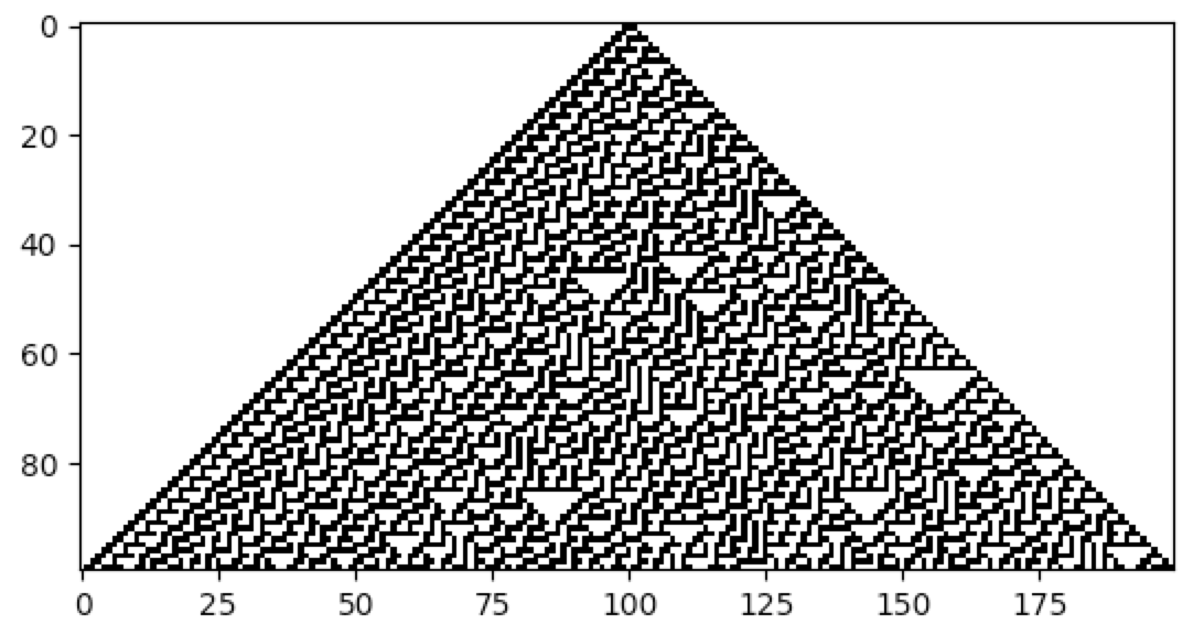
You should use CellPyLib if:

  • you are an instructor or student wishing to learn more about Elementary Cellular Automata and 2D Cellular Automata on a uniform grid (such as the Game of Life, the Abelian sandpile, Langton's Loops, etc.)
  • you are a researcher who wishes to work with Elementary Cellular Automata and/or 2D Cellular Automata on a uniform grid, and would like to use a flexible, correct and tested library that provides access to such models as part of your research

If you would like to work with Cellular Automata on arbitrary networks (i.e. non-uniform grids), have a look at the Netomaton project. If you would like to work with 3D CA, have a look at the CellPyLib-3d project.

Getting Started

CellPyLib can be installed via pip:

pip install cellpylib

Requirements for using this library are Python 3.6, NumPy, and Matplotlib. Have a look at the documentation, located at cellpylib.org, for more information.

Varying the Neighbourhood Size

The size of the cell neighbourhood can be varied by setting the parameter r when calling the evolve function. The value of r represents the number of cells to the left and to the right of the cell under consideration. Thus, to get a neighbourhood size of 3, r should be 1, and to get a neighbourhood size of 7, r should be 3. As an example, consider the work of M. Mitchell et al., carried out in the 1990s, involving the creation (discovery) of a cellular automaton that solves the density classification problem: if the initial random binary vector contains more than 50% of 1s, then a cellular automaton that solves this problem will give rise to a vector that contains only 1s after a fixed number of time steps, and likewise for the case of 0s. A very effective cellular automaton that solves this problem most of the time was found using a Genetic Algorithm.

import cellpylib as cpl

cellular_automaton = cpl.init_random(149)

# Mitchell et al. discovered this rule using a Genetic Algorithm
rule_number = 6667021275756174439087127638698866559

# evolve the CA, setting r to 3, for a neighbourhood size of 7
cellular_automaton = cpl.evolve(cellular_automaton, timesteps=149,
                                apply_rule=lambda n, c, t: cpl.binary_rule(n, rule_number), r=3)

cpl.plot(cellular_automaton)

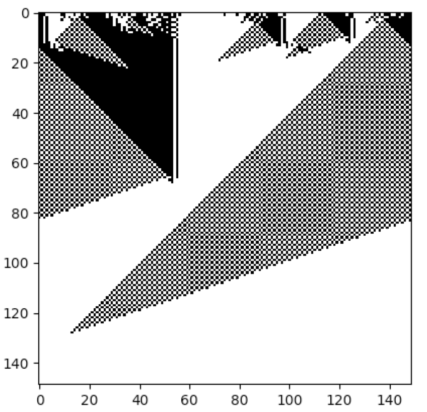
For more information, see:

Melanie Mitchell, James P. Crutchfield, and Rajarshi Das, "Evolving Cellular Automata with Genetic Algorithms: A Review of Recent Work", In Proceedings of the First International Conference on Evolutionary Computation and Its Applications (EvCA'96), Russian Academy of Sciences (1996).

Varying the Number of Colors

The number of states, or colors, that a cell can adopt is given by k. For example, a binary cellular automaton, in which a cell can assume only values of 0 and 1, has k = 2. CellPyLib supports any value of k. A built-in function, totalistic_rule, is an implementation of the Totalistic cellular automaton rule, as described in Wolfram's NKS. The code snippet below illustrates using this rule. A value of k of 3 is used, but any value between (and including) 2 and 36 is currently supported. The rule number is given in base 10 but is interpreted as the rule in base k (thus rule 777 corresponds to '1001210' when k = 3).

import cellpylib as cpl

cellular_automaton = cpl.init_simple(200)

# evolve the CA, using totalistic rule 777 for a 3-color CA
cellular_automaton = cpl.evolve(cellular_automaton, timesteps=100,
                                apply_rule=lambda n, c, t: cpl.totalistic_rule(n, k=3, rule=777))

cpl.plot(cellular_automaton)

Rule Tables

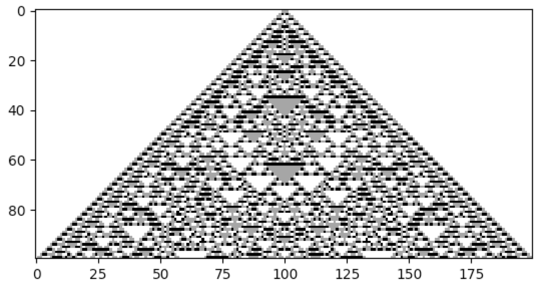
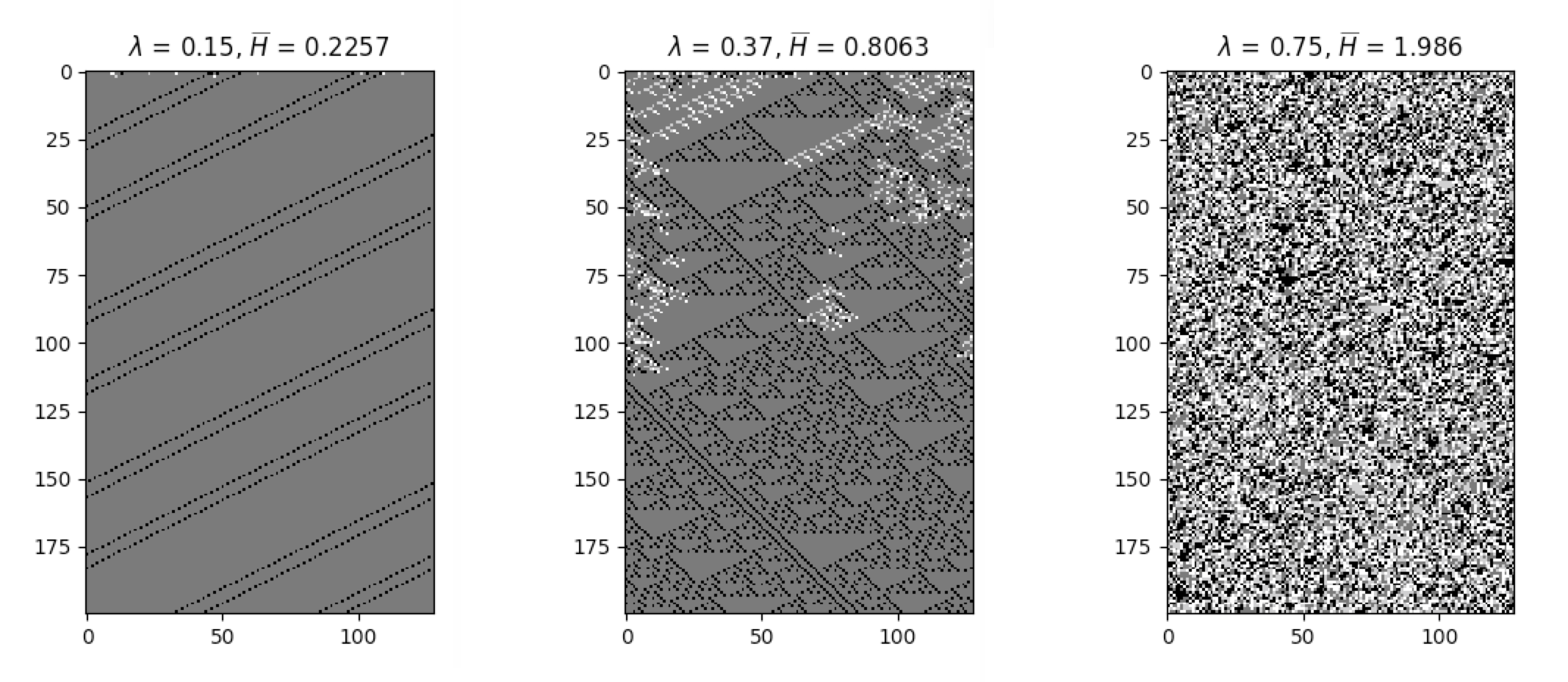
One way to specify cellular automata rules is with rule tables. Rule tables are enumerations of all possible neighbourhood states together with their cell state mappings. For any given neighbourhood state, a rule table provides the associated cell state value. CellPyLib provides a built-in function for creating random rule tables. The following snippet demonstrates its usage:

import cellpylib as cpl

rule_table, actual_lambda, quiescent_state = cpl.random_rule_table(lambda_val=0.45, k=4, r=2,
                                                                   strong_quiescence=True, isotropic=True)

cellular_automaton = cpl.init_random(128, k=4)

# use the built-in table_rule to use the generated rule table
cellular_automaton = cpl.evolve(cellular_automaton, timesteps=200,
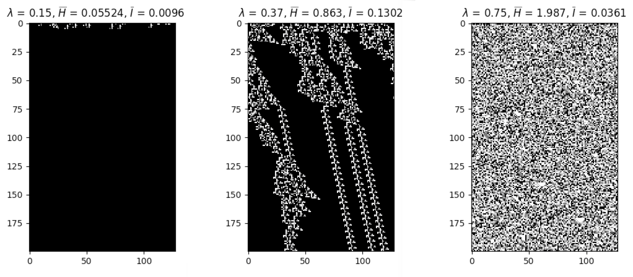
                                apply_rule=lambda n, c, t: cpl.table_rule(n, rule_table), r=2)

The following plots demonstrate the effect of varying the lambda parameter:

C. G. Langton describes the lambda parameter, and the transition from order to criticality to chaos in cellular automata while varying the lambda parameter, in the paper:

Langton, C. G. (1990). Computation at the edge of chaos: phase transitions and emergent computation. Physica D: Nonlinear Phenomena, 42(1-3), 12-37.

Measures of Complexity

CellPyLib provides various built-in functions which can act as measures of complexity in the cellular automata being examined.

Average Cell Entropy

Average cell entropy can reveal something about the presence of information within cellular automata dynamics. The built-in function average_cell_entropy provides the average Shannon entropy per single cell in a given cellular automaton. The following snippet demonstrates the calculation of the average cell entropy:

import cellpylib as cpl

cellular_automaton = cpl.init_random(200)

cellular_automaton = cpl.evolve(cellular_automaton, timesteps=1000,
                                apply_rule=lambda n, c, t: cpl.nks_rule(n, 30))

# calculate the average cell entropy; the value will be ~0.999 in this case
avg_cell_entropy = cpl.average_cell_entropy(cellular_automaton)

The following plots illustrate how average cell entropy changes as a function of lambda:

Average Mutual Information

The degree to which a cell state is correlated to its state in the next time step can be described using mutual information. Ideal levels of correlation are required for effective processing of information. The built-in function average_mutual_information provides the average mutual information between a cell and itself in the next time step (the temporal distance can be adjusted). The following snippet demonstrates the calculation of the average mutual information:

import cellpylib as cpl

cellular_automaton = cpl.init_random(200)

cellular_automaton = cpl.evolve(cellular_automaton, timesteps=1000,
                                apply_rule=lambda n, c, t: cpl.nks_rule(n, 30))

# calculate the average mutual information between a cell and itself in the next time step
avg_mutual_information = cpl.average_mutual_information(cellular_automaton)

The following plots illustrate how average mutual information changes as a function of lambda:

Reversible Cellular Automata

Elementary cellular automata can be explicitly made to be reversible. The following example demonstrates the creation of the elementary reversible cellular automaton rule 90R:

import cellpylib as cpl

cellular_automaton = cpl.init_random(200)
rule = cpl.ReversibleRule(cellular_automaton[0], 90)

cellular_automaton = cpl.evolve(cellular_automaton, timesteps=100, 
                                apply_rule=rule)

cpl.plot(cellular_automaton)

Continuous Cellular Automata

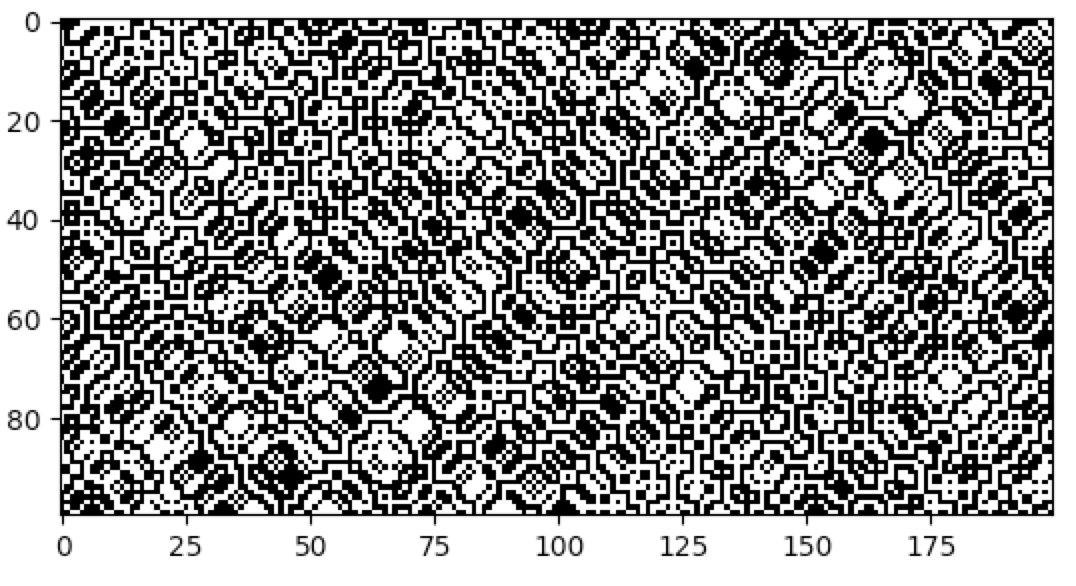
In addition to discrete values, cellular automata can assume continuous values. CellPyLib supports continuous-valued automata. To create cellular automata with continuous values--or any kind of data type--simply specify the dtype parameter when invoking any of the init and evolve built-in functions. For example, to create a cellular automata with continuous values, one might specify the following parameter: dtype=np.float32.

2D Cellular Automata

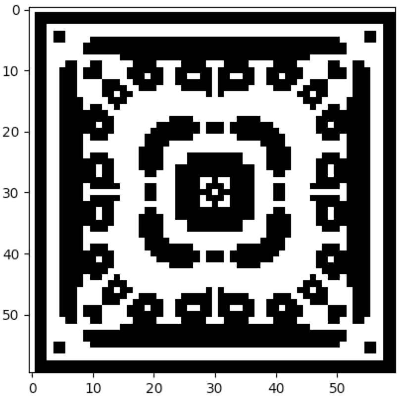
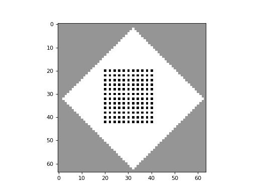
CellPyLib supports 2-dimensional cellular automata with periodic boundary conditions. The number of states, k, can be any whole number. The neighbourhood radius, r, can also be any whole number, and both Moore and von Neumann neighbourhood types are supported. The following snippet demonstrates creating a 2D totalistic cellular automaton:

import cellpylib as cpl

# initialize a 60x60 2D cellular automaton 
cellular_automaton = cpl.init_simple2d(60, 60)

# evolve the cellular automaton for 30 time steps, 
#  applying totalistic rule 126 to each cell with a Moore neighbourhood
cellular_automaton = cpl.evolve2d(cellular_automaton, timesteps=30, neighbourhood='Moore',
                                  apply_rule=lambda n, c, t: cpl.totalistic_rule(n, k=2, rule=126))

cpl.plot2d(cellular_automaton)

The plot2d function plots the state of the cellular automaton at the final time step:

Conway's Game of Life

There are a number of built-in plotting functions for 2D cellular automata. For example, plot2d_animate will animate the evolution of the cellular automaton. This is illustrated in the following snippet, which demonstrates the built-in Game of Life rule:

import cellpylib as cpl

# Glider
cellular_automaton = cpl.init_simple2d(60, 60)
cellular_automaton[:, [28,29,30,30], [30,31,29,31]] = 1

# Blinker
cellular_automaton[:, [40,40,40], [15,16,17]] = 1

# Light Weight Space Ship (LWSS)
cellular_automaton[:, [18,18,19,20,21,21,21,21,20], [45,48,44,44,44,45,46,47,48]] = 1

# evolve the cellular automaton for 60 time steps
cellular_automaton = cpl.evolve2d(cellular_automaton, timesteps=60, neighbourhood='Moore',
                                  apply_rule=cpl.game_of_life_rule, memoize='recursive')

cpl.plot2d_animate(cellular_automaton)

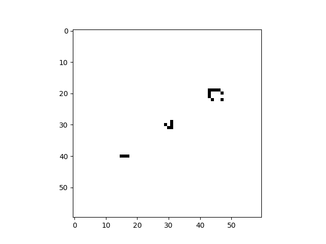
For more information about Conway's Game of Life, see:

Conway, J. (1970). The game of life. Scientific American, 223(4), 4.

Block Cellular Automata

Instead of a rule applying to a single cell at a time (given its neighbourhood), a rule can apply to a block of cells, given only the states of the cells in the block. Such a system is called a block cellular automaton. For example, the following code reproduces the block CA at the bottom of page 460 of Wolfram's NKS:

import cellpylib as cpl
import numpy as np

initial_conditions = np.array([[0]*13 + [1]*2 + [0]*201])

def block_rule(n, t):
    if n == (1, 1): return 1, 1
    elif n == (1, 0): return 1, 0
    elif n == (0, 1): return 0, 0
    elif n == (0, 0): return 0, 1

ca = cpl.evolve_block(initial_conditions, block_size=2, 
                      timesteps=200, apply_rule=block_rule)
cpl.plot(ca)

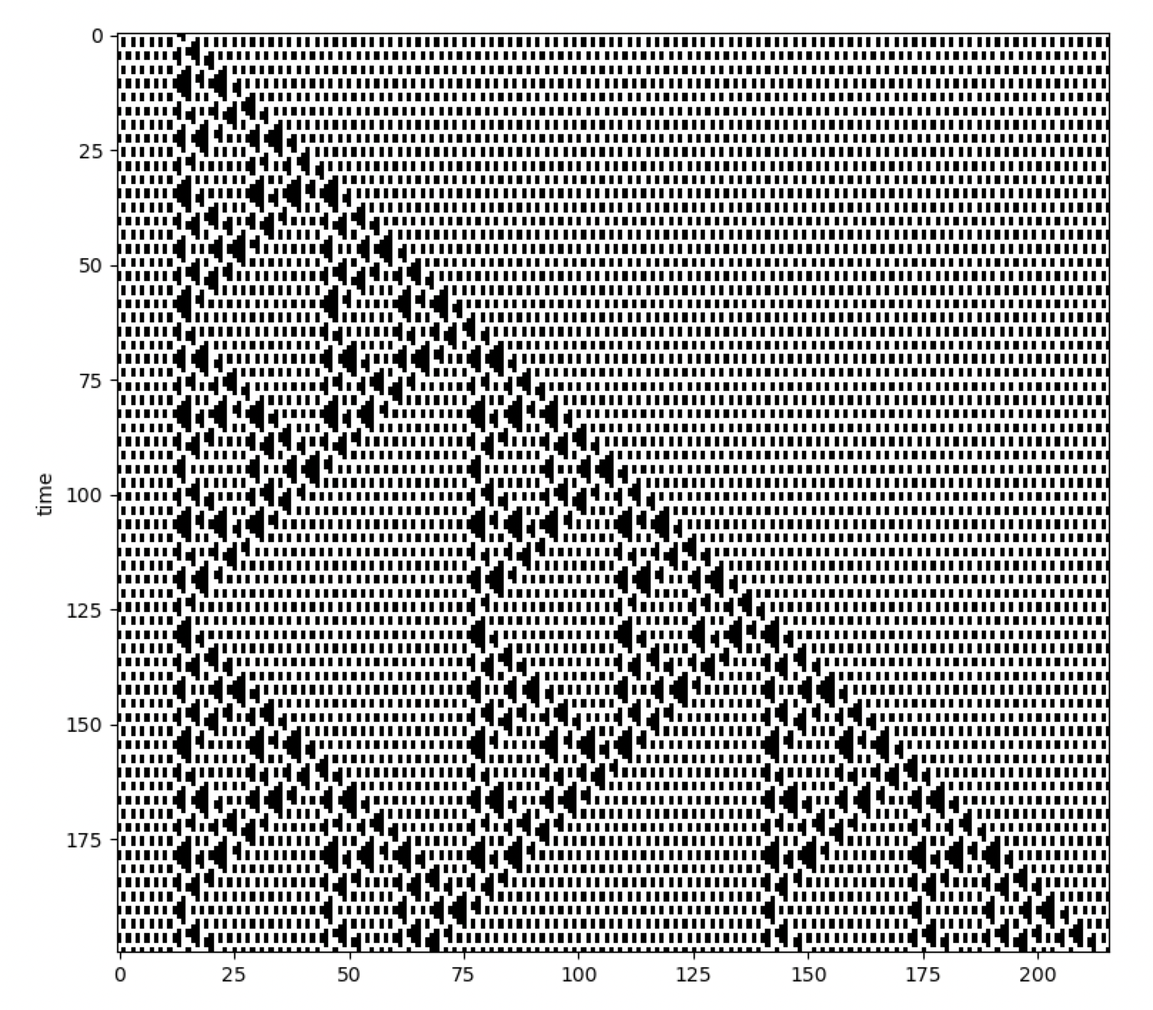
Block cellular automata can also exist in 2 dimensions, as the following example demonstrates:

The full source code for this example can be found here.

Increasing Execution Speed with Memoization

Memoization is expected to provide an increase to execution speed when there is some overhead involved when invoking the rule. Only stateless rules that depend only on the cell neighbourhood are supported. Consider the following example of rule 30, where memoization is enabled:

import cellpylib as cpl
import time

start = time.time()
cpl.evolve(cpl.init_simple(1000), timesteps=500,
           apply_rule=lambda n, c, t: cpl.nks_rule(n, 30), memoize=True)

print(f"Elapsed: {time.time() - start:.2f} seconds")

The program above prints Elapsed: 0.33 seconds (actual execution time may vary, depending on the device used). Without memoization, the program requires approximately 23 seconds to complete.


Development

Create a Conda environment from the provided environment YAML file:

$ conda env create -f environment.yml

Documentation

To build the Sphinx documentation locally, from the doc directory:

$ make clean html

The generated files will be in _build/html.

To build the documentation for publication, from the doc directory:

$ make github

The generated files will be in _build/html and in the site/docs folder.

Testing

There are a number of unit tests for this project. To run the tests:

$ python -m pytest tests

If the pytest-cov package is installed, a coverage report can be generated by running the tests with:

$ python -m pytest tests/ --cov=cellpylib

Support

If you have any questions or comments, or if you find any bugs, please open an issue in this project. Please feel free to fork the project, and create a pull request, if you have any improvements or bug fixes. We welcome all feedback and contributions.


Citation Info

This project has been published in the Journal of Open Source Software. This project may be cited as:

Antunes, L. M. (2021). CellPyLib: A Python Library for working with Cellular Automata. Journal of Open Source Software, 6(67), 3608.

BibTeX:

@article{Antunes2021,
  doi = {10.21105/joss.03608},
  url = {https://doi.org/10.21105/joss.03608},
  year = {2021},
  publisher = {The Open Journal},
  volume = {6},
  number = {67},
  pages = {3608},
  author = {Luis M. Antunes},
  title = {CellPyLib: A Python Library for working with Cellular Automata},
  journal = {Journal of Open Source Software}
}

Stars

Please star this repository if you find it useful, or use it as part of your research.

License

Apache License 2.0

cellpylib's People

Contributors

lantunes avatar

Stargazers

 avatar  avatar  avatar  avatar  avatar  avatar  avatar  avatar  avatar  avatar  avatar  avatar  avatar  avatar  avatar  avatar  avatar  avatar  avatar  avatar  avatar  avatar  avatar  avatar  avatar  avatar  avatar  avatar  avatar  avatar  avatar  avatar  avatar  avatar  avatar  avatar  avatar  avatar  avatar  avatar  avatar  avatar  avatar  avatar  avatar  avatar  avatar  avatar  avatar  avatar  avatar  avatar  avatar  avatar  avatar  avatar  avatar  avatar  avatar  avatar  avatar  avatar  avatar  avatar  avatar  avatar  avatar  avatar  avatar  avatar  avatar  avatar  avatar  avatar  avatar  avatar  avatar  avatar  avatar  avatar  avatar  avatar  avatar  avatar  avatar  avatar  avatar  avatar  avatar  avatar  avatar  avatar  avatar  avatar  avatar  avatar  avatar  avatar  avatar  avatar

Watchers

 avatar  avatar  avatar  avatar  avatar  avatar  avatar  avatar

cellpylib's Issues

[JOSS] Consider adding package to conda forge

As an alternative installation path to pip, anaconda is gaining traction. Have you considered adding cellpylib to conda-forge, such that it can be installed via conda install cellpylib? This may make it easier for users that have a conda-based setup (which is not uncommon among students, for instance).

Step-by-step instructions for contributing to conda forge can be found here. Once set up, maintenance work is minimal: A GitHub action regularly checks whether your main branch has changed and, if so, will update the package in conda โ€“ optionally, this can be done without any interaction from your side.

To be clear: This is merely a proposition, I do not see it as essential for the review to go forward.

[JOSS] Highlight target audience in documentation

As a last issue for the JOSS review (at least from my side), there is the following point to address in the documentation:

A statement of need: Do the authors clearly state what problems the software is designed to solve and who the target audience is?

The current version of the documentation is quite clear in describing what the software is designed to do. However, I think it could be improved by more clearly stating the target audience. While the information is there indirectly (people interested in working with the mentioned CAs), I'd like to suggest to add a paragraph that directly addresses the target audience and answers the question of why they should use CellPyLib (and in which cases an alternative may be more appropriate).

I think that a condensed version of the section you use in the software paper could be very helpful to have on the landing page of the documentation. Maybe a short list of bullet points (e.g. "You should use CellPyLib if...") would also suffice.

[JOSS] Documentation issues

The documentation of certain functions is in my opinion insufficiently detailed. There are a number of functions implementing concepts that I was not familiar with. The documentation does not explain these concepts. Instead, it simply references some papers or arXiv preprints. I feel that having to read a paper to understand what a function does is too big an ask, especially when the function can be implemented in less than 10 lines.

I think that all functions in bien.py could benefit from better documentation, and a brief explanation of what is being calculated.

[JOSS] Update copyright section of README

In the Copyright section of the README you currently state "All rights reserved". I am not a lawyer, but in the context of Open Source Software this may introduce some confusion because the phrase appears to be obsolete (for the purpose of establishing copyright) and you license the software under the Apache license anyway, somewhat contradicting the statement.

Propositions:

  • If you are fine with it, remove the "All rights reserved" phrase
  • Update the year in the copyright notice
  • Somewhere in the README mention that cellpylib is open source software and refer to the license file

[JOSS] Namespace is polluted with symbols that shouldn't be there

Python is not my main language, so it is entirely possible that the "problem" I will mention here is not really considered a problem in the Python community. However, I do not see this issue in polished Python packages.

It is generally convenient to explore a package through the autocompletion feature of Jupyter or your IDE. Thus I like to type cpl., hit tab, and see what is in that namespace. I see a lot of things that do not belong there, such as np (from import numpy as np or Axes3D (which comes from matplotlib).

IMO a polished package should control explicitly which symbols are exported and made public.

It is now not clear if the functions I mentioned in #8 are even intended to be public (probably not).

[JOSS] Questions

This is not a bug report, just a means to ask questions @lantunes, for the purpose of the JOSS review. I hope it is okay to do it here. If not, can you please point me to a better location (perhaps there's a support forum)?

[JOSS] Cross-reference functions in documentation

First off: what I've read of the documentation so far is very nicely written ๐Ÿ‘

I think what would further improve it would be cross-references to the API documentation. For instance, in working.rst, a link to init_simple would be very useful, I think, as it allows to check out the function signature and other available arguments.

You already have the API reference as part of your documentation via automodule, if I see it correctly. To reference to it, you can use the domain syntax. For instance, :py:func: can be used to reference a function:

The initial conditions are instantiated using the function
:py:func:`~cellpylib.ca_functions.init_simple`, which, in this example ...

which yields a link to the API docs when rendered:

Screenshot 2021-09-24 at 16 08 50

I would propose to do this across all of the docs, as it really reduces friction, makes the functions stand out more, and makes the docs overall more useful. I think this could be applied semi-automatically across many files of the docs using search-and-replace, such that workload does not go over the top?

Plotting animation issue in Spyder IDE

Plotting the animations from CPL in Spyder IDE does not work for me. Using cpl.plot2d_animate()

The issue I get:

UserWarning: Animation was deleted without rendering anything. This is most likely unintended. To prevent deletion, assign the Animation to a variable that exists for as long as you need the Animation.
warnings.warn(

Relates to these issues:

I can get other animations to work, such as matplotlib simple animation: https://matplotlib.org/2.0.2/examples/animation/simple_anim.html

Perhaps there is something in the cpl.plot2d_animate function that is missing or should be returning an object?

Code used:

` # Glider
cellular_automaton = cpl.init_simple2d(60, 60)
cellular_automaton[:, [28,29,30,30], [30,31,29,31]] = 1

# evolve the cellular automaton for 60 time steps
cellular_automaton = cpl.evolve2d(cellular_automaton, timesteps=60, neighbourhood='Moore',
                                  apply_rule=cpl.game_of_life_rule, memoize='recursive')

# None of these matplotlib commands really solve the issue:
# %matplotlib qt5
# %matplotlib qt4
# %matplotlib inline

anim = cpl.plot2d_animate(cellular_automaton, interval=50, save=False)`

[JOSS] Use of deprecated `np.int`

Running the tests emits a large number (>600) of warnings, most of which stem from the use of np.int in the init_โ€ฆ functions. np.int is simply an alias to the builtin Python int and โ€“ as of numpy 1.20 โ€“ np.int is deprecated.

You can simply replace it with int to address the warnings. Alternatively, you may want to use the precision limited (but perhaps faster) np.int64, np.int32โ€ฆ

[JOSS] Plotting-related questions and suggestions

I'm unsure how expansive the plotting functionality of this package is meant to be and what its aim is. For instance, is it meant to be used for producing publication-ready plots? Or rather as a set of useful functions during the exploratory phase of a CA?
Can you briefly comment on that, @lantunes?

Expanding on #12, I have a few suggestions regarding the plotting functionality of cellpylib; depending on your comment to the above, these may or may not apply.


1 - Pass on arguments to underlying plotting function

This would make the plotting functions much more flexible, as it allows to pass on arguments to plt.imshow:

def plot(ca, title='', *, cmap='Greys', **imshow_kwargs):
    plt.title(title)
    plt.imshow(ca, interpolation='none', cmap=cmap, **imshow_kwargs)
    plt.show()

While not super relevant for the (short) plot function, larger functions like plot2d_animate would benefit from that, imo.

2 - Allow for non-interactive use (or document that this is not possible)

Afais, all plot functions end in plt.show(). If called in a script (like those in demos/), this leads to the interactive matplotlib window appearing, requiring user interaction.

This prohibits automation for saving plots, because the appearing plot windows need to be manually closed for the script to continue running. Example scenario: Making a bunch of different instantiations of a stochastic CA and their evolution and intending to save all of the resulting plots or animations.

I see the appeal of the current implementation of the plot function, especially when interactively working with the library. However, I think the plots always being shown unnecessarily restricts the plotting functions to these interactive use cases.

Proposition: Add another keyword argument (show=True) which can be set to False if working non-interactively. Alternatively, add a module-level variable that controls the default behaviour (but this is a tad more complicated to coordinate, probably overkill).

[JOSS] Use `__call__` magic method for rule classes

A suggestion that would make the use of rule classes like ReversibleRule more concise: Implement a __call__ magic method, such that the following syntax becomes possible:

ca = cpl.init_random(200)
my_rule = cpl.ReversibleRule(ca[0], 90)

ca = cpl.evolve(ca, timesteps=100, apply_rule=my_rule)  # NOTE: Without .apply_rule

Implementation would be:

class ReversibleRule:
    def __init__(self, init_state, rule_number):
        self._previous_state = init_state
        self._rule_number = rule_number

    def __call__(self, n, c, t):
        regular_result = nks_rule(n, self._rule_number)
        new_result = regular_result ^ self._previous_state[c]
        self._previous_state[c] = n[len(n) // 2]

        return new_result

In my mind, this not only simplifies the interface but also represents a clearer model of what a rule is: a callable that propagates the CA state.

Two further suggestions in that context:

  • I would propose to add a section to the docs, perhaps under "additional features" that illustrates how to implement a stateful rule like the ReversibleRule, such that users of CellPyLib can themselves define more advanced rules.
  • In case you intend to go towards more complex rule classes, you could consider providing a BaseRule class from which users can derive their own rule implementations. Such a base class may provide the interface (abstract __call__ method) and provide a template for expansion.

What do you think?

Neighbourhood

Hello! First of all thanks for this great library. It's very helpful as I have only started working with automata. I would like to ask whether its possible to define my own neighborhood and not use neither Moore nor von Neummann. Thank you.

[JOSS] Wishlist: Colormap support and feature parity for plotting functions

As far as I can tell, plot2d_animate is the only plotting function that has colormap support. With cellular automata that operate with a small and fixed number of discrete states, it is very useful to be able to assign a specific colour to each state. Thus, it would be nice to have this feature for all plotting functions, both for the 1D and 2D cases.

I notice that plot2d_animate has a bunch of other visualization settings that could also be ported to other plotting functions, such as show_grid.

[JOSS] Wishlist: Visualizing rules

Feature idea: Visualizing rules.

Currently, CellPyLib seems to be a very nice tool for learning / teaching about cellular automata. It can simulate many classic models. To expand its usability for this purpose, it would be nice to have functions for visualizing deterministic update rules, in the spirit of Mathematica's RulePlot.

Here are a few examples of what Mathematica's RulePlot does, for inspiration:

Rule 30:

image

3-colour rule 123:

image

A two-dimensional case:

image

As you can see, it lists all possible neighbourhoods, and shows how the cell would get updated.

Evolve should accept CA with prior history

Currently, the evolve and evolve2d functions assume the initial conditions consist of just the first timestep, and start from the first (and only) state of the given initial conditions list. However, it would be convenient if a user could supply a list of multiple states, representing some prior evolution history, and the evolve and evolve2d functions could continue from the last state in the list.

Error when trying to use a neighborhood of size 4 (r=1.5)

Hi, I am trying to test the evolution of the automaton with a neighborhood of size 4 given by r=1.5, but I get the following error:

TypeError: slice indices must be integers or None or have an __index__ method

This is the code to reproduce it:

cellular_automaton = cpl.init_random(8)
rule_number = 73
cellular_automaton = cpl.evolve(cellular_automaton, timesteps = 6,
                                apply_rule = lambda n, c, t: cpl.binary_rule(n, rule_number, scheme='nks'),  r = 1.5)
print(cellular_automaton)

Attached is also an image of the error:

image

Increasing performance

Hi there and thanks for the intuitive library!

I'd like to recreate the experiments from the paper you mention in the readme: "Evolving Cellular Automata with Genetic Algorithms: A Review of Recent Work" from Melanie Mitchell, James P. Crutchfield, and Rajarshi Das. However, evolving a population of say 100 automata for some generations takes quite a while.

Profiling showed one simple way to reduce the runtime: In binary_rule the rule is given as an int and converted to bits using the int_to_bits method in every call. Storing the rule as bits and skipping the conversion reduced the runtime of my experiments. Is there a way to support this in the library? I'm thinking of a possibility to simply hand a binary np-array into the binary_rule method, see exemplary code below.

The same goes with the bits_to_int method. After profiling with above code this is the method causing the most runtime. A possible performance improvement would be to calculate the powers of 2 beforhand and then only compute the dot product of neighbourhood and the powers of 2 as suggested here.

I've sketched both perfomance improvements in a fast_binary_rule method:

def fast_binary_rule(neighbourhood, binary_rule, powers_of_two, scheme=None):
    state_int = neighbourhood.dot(powers_of_two)
    n = 2 ** len(neighbourhood)
    if scheme == 'nks':
        return binary_rule[(n - 1) - state_int]
    return binary_rule[state_int]

The usage is pretty much the same but with the additional powers_of_two parameter. Here a full example:

import cellpylib as cpl
import numpy as np


def fast_binary_rule(neighbourhood, binary_rule, powers_of_two, scheme=None):
    state_int = neighbourhood.dot(powers_of_two)
    n = 2 ** len(neighbourhood)
    if scheme == 'nks':
        return binary_rule[(n - 1) - state_int]
    return binary_rule[state_int]


timesteps = lattice_size = 49
neighbourhood_radius = 3
powers_of_two = a = 2 ** np.arange(neighbourhood_radius * 2 + 1)[::-1]

cellular_automaton = cpl.init_random(lattice_size)

rule = np.random.choice([0, 1], size=(128,))

cellular_automaton = cpl.evolve(cellular_automaton, timesteps=timesteps,
                                apply_rule=lambda n, c, t: fast_binary_rule(n, rule, powers_of_two),
                                r=neighbourhood_radius)

cpl.plot(cellular_automaton)

On my machine using the fast_binary_rule cuts the execution time of my experiments roughly in half. Would you be interessted in integrating these performance improvements?

And: Are there other performance improvements to further reduce runtime?

[JOSS] Report (and improve) test coverage

Running python -m pytest tests/ --cov=cellpylib (with pytest-cov package installed) currently yields the following coverage report:

---------- coverage: platform darwin, python 3.9.6-final-0 -----------
Name                          Stmts   Miss  Cover
-------------------------------------------------
cellpylib/__init__.py             9      0   100%
cellpylib/apen.py                17      1    94%
cellpylib/bien.py                45      0   100%
cellpylib/ca_functions.py       133     17    87%
cellpylib/ca_functions2d.py     119     69    42%
cellpylib/ctrbl_rule.py          27      0   100%
cellpylib/entropy.py             35      1    97%
cellpylib/hopfield_net.py        28      0   100%
cellpylib/langtons_loop.py      121    116     4%
cellpylib/rule_tables.py         74      6    92%
-------------------------------------------------
TOTAL                           608    210    65%

Wide parts of the library seem to be well-covered and most of the missing statements come from the (rather complicated) langtons_loop module. However, I would expect a higher test coverage in the two ca_functions modules, given that they are the core part of the library.

@lantunes Have you checked which of the statements are currently untested and would you consider expanding the corresponding tests to cover wider parts of the core library?

[JOSS] Changelog is not available

The past releases do not provide a changelog, see https://github.com/lantunes/cellpylib/releases

If this software is to be relied upon by researchers, I strongly suggest to start providing changelogs going forward (or even back to version 1.0.0, which I assume marks the beginning of a stable API?).

On a related note, does versioning follow semver? If yes, it is useful to mention this.

[JOSS] Consider adding axis labels to 1D plots

While I have worked with 2D CA a lot, I'm not particularly used to 1D CA and it seems to me that there are different conventions for which axis is associated with time and space. What do you think about automatically adding axis labels (x and time) to the 1D CA plots?

The signature could be:

def plot(ca, title='', *, add_labels=True):
    # ...

For consistency, I would propose to implement the same functionality in all plot functions, but maybe use a different default; for animations of 2D CAs the labels are less relevant, imo.

[JOSS] Minor tweaks to references in paper.md

Hi @lantunes, I'm here as one of the reviewers from your submission to JOSS ๐Ÿ‘‹

I just read the paper (before looking into the code) and have only minor remarks regarding the references:

  1. In the first paragraph, the two successive citations can be combined like this:
... Deep Learning [@nichele2017deep,@mordvintsev2020growing] ...
  1. I think it would be more appropriate to mark up the title of the Wolfram book as italic (as done in the references) rather than verbatim. Just a suggestion, though.

  2. For the Mordvintsev et al. citation, they supply the following BibTeX on their webpage, which includes a DOI (that @whedon must have missed):

@article{mordvintsev2020growing,
  author = {Mordvintsev, Alexander and Randazzo, Ettore and Niklasson, Eyvind and Levin, Michael},
  title = {Growing Neural Cellular Automata},
  journal = {Distill},
  year = {2020},
  note = {https://distill.pub/2020/growing-ca},
  doi = {10.23915/distill.00023}
}
  1. Did you check if there are DOIs available for the Wolfram and von Neumann books? (There sometimes are, but if not, no worries.)

Let me know if there are questions or if I can assist with anything.

Definition of AsynchronousRule

First of all thanks for this project, it's been great for beginners such as I who are getting to learn about automata!

I'm trying to understand how the AsynchronousRule works. The demo works nicely but I'm not sure how to configure it to prioritize certain neighbours over others. In the demo, the priority seems ranked by the position of the cell, right?

But what if one wanted to prioritize the neighbourhood by value instead? That is, all the combinations of ranks for the possible neighborhoods of the elementary space, which is a tuple of length 8, each element representing a rank between 1 and 7, inclusive.

I feel like it's still related to update_order parameter, but it's different in the sense that it's not the the same async-update strategy (one is positional and the other is by cell-state). Does this make sense?

Recommend Projects

  • React photo React

    A declarative, efficient, and flexible JavaScript library for building user interfaces.

  • Vue.js photo Vue.js

    ๐Ÿ–– Vue.js is a progressive, incrementally-adoptable JavaScript framework for building UI on the web.

  • Typescript photo Typescript

    TypeScript is a superset of JavaScript that compiles to clean JavaScript output.

  • TensorFlow photo TensorFlow

    An Open Source Machine Learning Framework for Everyone

  • Django photo Django

    The Web framework for perfectionists with deadlines.

  • D3 photo D3

    Bring data to life with SVG, Canvas and HTML. ๐Ÿ“Š๐Ÿ“ˆ๐ŸŽ‰

Recommend Topics

  • javascript

    JavaScript (JS) is a lightweight interpreted programming language with first-class functions.

  • web

    Some thing interesting about web. New door for the world.

  • server

    A server is a program made to process requests and deliver data to clients.

  • Machine learning

    Machine learning is a way of modeling and interpreting data that allows a piece of software to respond intelligently.

  • Game

    Some thing interesting about game, make everyone happy.

Recommend Org

  • Facebook photo Facebook

    We are working to build community through open source technology. NB: members must have two-factor auth.

  • Microsoft photo Microsoft

    Open source projects and samples from Microsoft.

  • Google photo Google

    Google โค๏ธ Open Source for everyone.

  • D3 photo D3

    Data-Driven Documents codes.