Automated identification of ontological terms in application area specific literature surveys

• You will need python version 3.4.2 or newer versions to execute the software.
• The project also depends on some other modules such as bibtexparser 0.6.2 and Inflect 0.2.5. Happily, these will be installed automatically when following the commands below.
• We use EXTRACT 2.0, a custom named entity recognition (NER) system to annotate the text contets with ontological terms.

Step 1: Cloning the repository

Here you will download a copy of the code and place it somewhere in your directory.

$ mkdir repos
$ cd repos
$ git clone https://github.com/KociOrges/pytag

Step 2: Installing the software using the setup.py file

$ cd pytag
$ python setup.py install

Step 3: Modify your search paths

By default, pytag will be installed in the site-packages and bin directory of your python version. For this reason, you need to set your $PATH appropriately so that the software can be executed. Make sure that you have the following path added in your $PATH:

/.pyenv/versions/3.X(>=4).Y(>=2)/bin

Once that is done, you can start annotating BibTex files from the command line. We will assume that you already have the BibTex files that you want to annotate in the directory path_to_BibTex_files/. We will also assume that you want to identify terms utilizing all the supported ontologies for your annotation. The identified terms are then described in the TSV table ontology_terms.tsv. This can be done as follows:

$ pytag --input_dir path_to_BibTex_files/ --onto_types all --out_file ontology_terms.tsv

You can also specify the ontology/ies that you want to utilise for your annotation by using the associated numerical identifiers as decribed below:

• 0: Genes/proteins from the specified organism
• -1: Small Molecule Compound identifiers
• -2: NCBI Taxonomy entries
• -21: Gene Ontology biological process terms
• -22: Gene Ontology cellular component terms
• -23: Gene Ontology molecular function terms
• -25: BRENDA Tissue Ontology terms
• -26: Disease Ontology terms
• -27: Environment Ontology terms

For example, let's say that you would like to identify the Environmental, Tissue and Disease mentions in your BibTex files. This can be done as follows (the order of the numerical identifiers is irrelevant):

$ pytag --input_dir path_to_BibTex_files/ --onto_types -27 -25 -26 --out_file ontology_terms.tsv

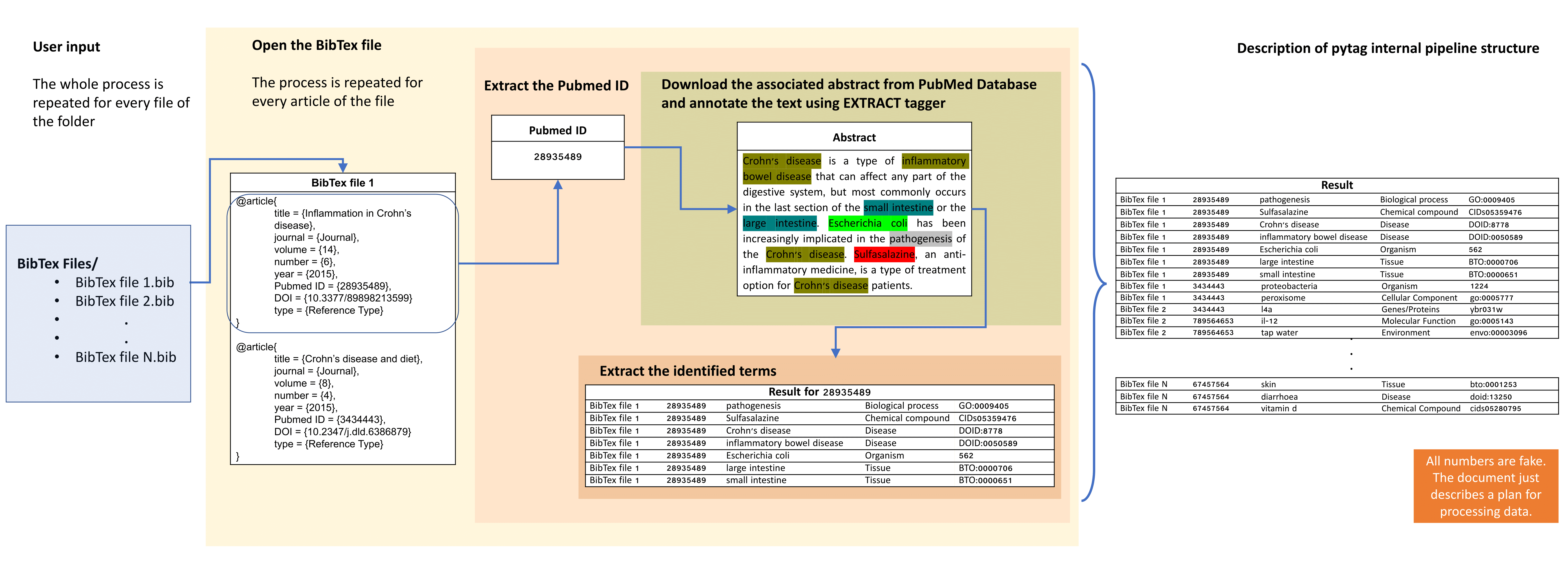
Starting from a keyword search in PubMed database, the returned abstracts can be extracted and then imported into a citation management software, such as EndNote. Next, they are exported in BibTeX format, where every reference is annotated with a number of records including PubMed IDs. In pyTag pipeline, for each PubMed ID described in the BibTex files, the associated link in NCBI database is followed and the relevant abstract is extracted. Next, these abstracts are processed using a custom named entity recognition (NER) system called EXTRACT 2.0. The system supports multiple ontologies and can recover the genes/proteins, small molecule compounds, organisms, environments, tissues, diseases, phenotypes and Gene Ontology terms in a given piece of text. After the collection and the annotation of the total number of abstracts is performed, a table describing the identified ontological terms is generated, which can next be subjected to statistical analysis for further exploration.

The volume of biomedical literature in electronic format has grown exponentially over the past few years. To explore this huge amount of data to reveal hidden patterns, there is a need to use automated textmining tools that can elucidate useful insights provided if the information is available in a structured format. With ontology-driven annotation of biomedical data gaining popularity in recent years and online databases offering metatags with rich textual information, it is now possible to textmine ontological terms and explore these aspects through downstream statistical analysis. The automated interpretation of literature data offered from pytag, can reduce the amount of information to manageable set of deducable patterns from which it is easier to draw conclusions and can be helpful for systematic reviews. See associated paper (Koci et al. 2018, https://doi.org/10.7717/peerj.5047).

Schematic of the workflow for the automated identification and analyses of ontological terms in literature data using pytag:

Schematic overview of pytag internal pipeline structure:

If you use pytag in your publication, please cite:

Koci O, Logan M, Svolos V, Russell RK, Gerasimidis K, Ijaz UZ. 2018. An automated identification and analysis of ontological terms in gastrointestinal diseases and nutrition-related literature provides useful insights. PeerJ 6:e5047 https://doi.org/10.7717/peerj.5047

We will run pytag using some BibTex files generated from keyword searches in PubMed database. Let's say that we are interested in exploring the content of ontological terms for publications related to Coeliac and Crohn's Disease and Ulcerative Colitis that cover aspects related to Nutrition, using the keywords: Diet, Food & Nutrition. This is all done for a time frame from 1991 to 2016 in pairs of years (1991-1992, 1993-1994 and so on). For that purpose, in PubMed database we have searched for the Boolean keywords: (Coeliac AND Diet/Food/Nutrition) (similarly for the other disease conditions) between 1991 to 2016, to obtain the relevant literature. For each search, we have labelled and extracted the citations in external files, using the “Citation Manager” function in MEDLINE (tagged) format. Next, we have imported these files into EndNote, to export them in BibTeX format where every reference is described with an associated PubMed ID. The PubMed ID is a unique identifier used in PubMed and assigned to each article record when it enters the PubMed system. Before we run pytag, we will need to make sure that our BibTex files contain in each of their references a record called Pubmed ID or Accession Number describing this unique identifier. You can find a tutorial on how to edit the bibliographic styles in EndNote here. The references in the BibTex files should look like this:

@article{
   title = {Latest evidence on Crohn's Disease}, 
   journal = {Journal},
   volume = {14},
   number = {6},
   ...
   Pubmed ID = {27483748}, 
   DOI = {10.8902/h.kldu.2015.04.017},
   year = {2015},
   type = {Reference Type}
}
*The details of the article are all fake. This example just describes how BibTex files should look like before processing.

Here, we have put the generated BibTex files for each keyword searched inside the folder tutorial/bibtex_example/.

$ cd tutorial/
$ ls bibtex_example/
Coeliac.Diet.1991.1992.bib			Crohn.Food.2005.2006.bib
Coeliac.Diet.1993.1994.bib			Crohn.Food.2007.2008.bib

In our scenario, we assume that we are interested in annotating our literature with terms that are related to all the supported ontology types (in case we would like to specify only some particular types then we should replace the parameter 'all' with the relevant numerical identifiers as described in section Usage). We also define ontology_terms.tsv as the TSV file where the identified terms will be described. This can be done as follows:

$ pytag --input_dir bibtex_example/ --onto_types all --out_file ontology_terms.tsv

As the script is running, in the output you should be able to see which file is currently being annotated and for the references that no terms were identified in their abstract text content, a relevant message with their associated PubMed ID is also shown on the command line. After a BibTex file is processed, then the total number of references, the number of availabe and annotated abstracts are mentioned for the specific file. When the execution is completed for all the BibTex files, then the total number of references processed, the total number of the annotated abstracts and the number of BibTex files annotated from the pipeline are also shown on the command line:

$ pytag --input_dir bibtex_example/ --onto_types all --out_file ontology_terms.tsv
Processing file: 1 Coeliac.Diet.1991.1992.bib
no annotation for reference with Pubmed ID:  1444165
Coeliac.Diet.1991.1992 : 185 references found in total. 159 abstracts were annotated from 160 available.
...
Crohn.Nutrition.2007.2008 : 256 references found in total. 216 abstracts were annotated from 226 available.
Processing file: 75 Crohn.Nutrition.2009.2010.bib
...
UlcerativeColitis.Nutrition.2015.2016 : 463 references found in total. 429 abstracts were annotated from 443 available.
Total number of references:  20549
Total number of annotated abstracts:  17750
Total number of BibTex files:  117

Once the pipeline has finished processing, you will have the following contents in your home folder:

$ ls
bibtex_example
ontology_terms.tsv
annotation_summary.tsv

The ontology_terms.tsv is the most interesting file and contains the ontology terms identified in the references of each BibTex file, followed with the associated PubMed ID of the abstract they were found in each case. For each term, the relevant ontology entry is mentioned followed with the associated identifier. The TSV file should look like this:

$ head ontology_terms.tsv
Coeliac.Diet.1991.1992	1452072		major histocompatibility	Biological Process	go:0046776	
Coeliac.Diet.1991.1992	1452072		lamina propria			Tissue			bto:0002330	
Coeliac.Diet.1991.1992	1452072		pathogenesis			Biological Process	go:0009405	
Coeliac.Diet.1991.1992	1452072		v 13				Chemical Compound	cids71299337	
Coeliac.Diet.1991.1992	1452072		bowel				Tissue			bto:0000648	
Coeliac.Diet.1991.1992	1452072		lymphocytes			Tissue			bto:0000775	
Coeliac.Diet.1991.1992	1452072		epithelial			Tissue			bto:0000416	
Coeliac.Diet.1991.1992	1452072		coeliac disease			Disease			doid:10608	
Coeliac.Diet.1991.1992	1452072		mucosal				Tissue			bto:0000886	
Coeliac.Diet.1991.1992	1452072		jejunal				Tissue			bto:0000657
...

In the annotation_summary.tsv table you will find for each BibTex file, the number of references that were found, the number of the abstracts that were available for these references and the number of the abstracts that were finally annotated. The file should look like this:

$ head annotation_summary.tsv 
			Total_number_of_references	Available_abstracts	Annotated_abstracts
Coeliac.Diet.1991.1992			       185			160			159
Coeliac.Diet.1993.1994			       139			122			122
Coeliac.Diet.1995.1996			       197			168			162
...

After the steps above are completed, then we can easily import the file with the identified ontological terms into R software and perform statistical analysis. First, we will need to source the associated Scripts for the analysis, and then import the table with the identified terms as well as the table with the annotation summary. This can be done as follows:

library(R.utils)
sourceDirectory("Rscripts/")

onto_terms <- read.delim("ontology_terms.tsv", header = FALSE, quote = "", 
                         row.names = NULL, 
                         stringsAsFactors = FALSE)
			 
colnames(onto_terms) <- c("Keyword", "PID", "Term", "Ontology", "Identifier")

annot_sum <- read.delim("annotation_summary.tsv", header = TRUE, row.names = 1)

To start our analysis, the next important step is to create the frequency table from the list of the identified terms. In our annotation example, we have used all the ontology types supported from the system. However, in our downstream statistical analysis we may be interested in exploring the content of terms from specific ontologies at a time. For example, in this case, we will extract and explore the terms that describe Organisms and Chemical compounds. This can be easily done as follows by adjusting the ontology parameter appropriately (in case we would like to include all types, then parameter ‘all’ should be used):

unique(onto_terms$Ontology)
[1] "Biological Process" "Tissue" "Chemical Compound" "Disease"     
[5] "Genes/Proteins" "Organism" "Molecular Function" "Cellular Component"
[9] "Environment"

freq_table <- create_frequency_table(onto_terms, ontology = c("Organism", "Chemical Compound"))

In addition, imagine that we have a meta table (tutorial/meta_table.tsv) that contains categorical information about the disease condition, the keyword type for nutrition and the date each search was performed on (where CCD: Coeliac Disease; CD: Crohn’s Disease; UC: Ulcerative Colitis). We can load the file like this:

meta_table <- read.delim("meta_table.tsv", header = TRUE, row.names = 1, stringsAsFactors = FALSE)

We may find also useful in our analysis to remove first any low count terms, e.g. terms with <= 5 hits across all searches. Then, we can normalise our data before doing statistics. To account for the variation of the publications over time and perform analysis in a longitudinal setting, we can normalise the counts of the terms of each search with respect to the number of the abstracts that were annotated for that search. This can be achieved by using the information given in the annotation_summary.tsv file (generated when annotation is performed) and using the script described below:

freq_table <- freq_table[, colSums(freq_table) > 5]
freq_table_norm <- normalise_data(freq_table, annot_sum, by = "Annotated_abstracts")

Significance of variability of ontological terms can be explored in a spatial (distances between groups) or temporal setting (expressed as in pairs of years) using permutation analysis of variance (PERMANOVA) and particularly, the function adonis from VEGAN package. All we need to do in such a case, is to specify the variables (Disease and/or Date) to be included in the formula and then obtain the corresponding r-squared (% of variability explained) and p-values.

library(vegan)
adonis(formula = freq_table_norm ~ Group + Date, data = meta_table)

Call:
adonis(formula = freq_table_norm ~ Group + Date, data = meta_table) 

Permutation: free
Number of permutations: 999

Terms added sequentially (first to last)

           Df SumsOfSqs MeanSqs F.Model      R2 Pr(>F)    
Group       2    8.5457  4.2729 29.9503 0.28095  0.001 ***
Date       12    7.3195  0.6100  4.2754 0.24064  0.001 ***
Residuals 102   14.5519  0.1427         0.47841           
Total     116   30.4171                 1.00000           
---
Signif. codes:  0 ‘***’ 0.001 ‘**’ 0.01 ‘*’ 0.05 ‘.’ 0.1 ‘ ’ 1

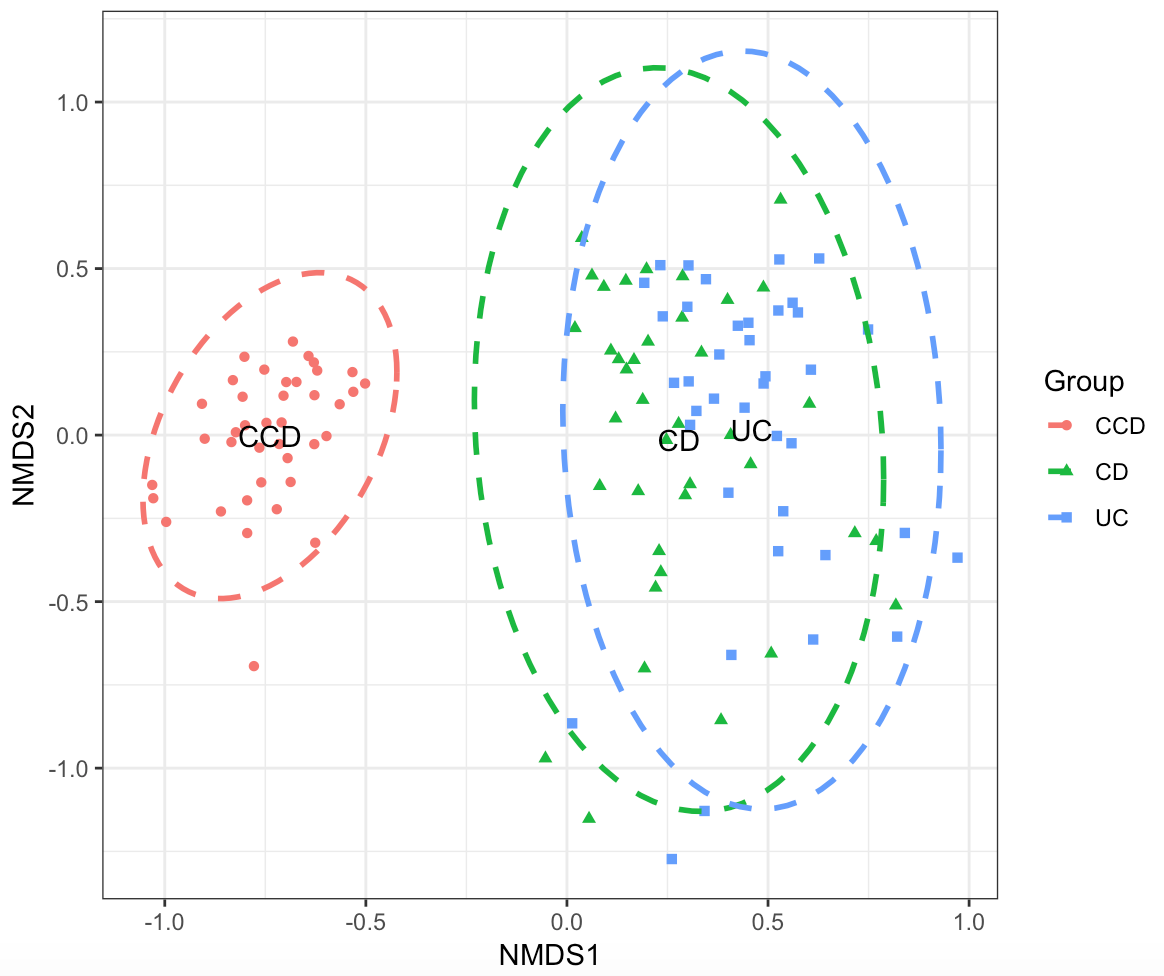
We can use Ordination to investigate for clustering between the disease groups i.e., how dissimilar the terms for a given search (disease condition or year) are from each other. Non-metric multidimensional scaling (NMDS) can be useful in this case, which simplifies the multivariate dataset into a just few dimensions (2D space, similar to PCA) based on dissimilarity (Bray-Curtis distance) between the terms for a given search. We perform NMDS analysis and visualise the result using the scripts as shown below:

nmdsres <- ordination_nmds(freq_table_norm, meta_table)
p <- plot_ordination(nmdsres, grouping_column = "Group", use_ellipse = TRUE, ell.kind = "sd")

One of the first things that can be interesting to observe is the ontological terms that are the most frequent in the literature of the investigated conditions. For example, we may be interested in visualising the top 20 terms in literature for the entire time frame or for a particular time range as described below:

p <- plot_frequent_terms(freq_table_norm, meta_table, grouping_column = "Group", range = "2001 - 2016", terms = 20)

Ontological terms that differentiate significantly between the disease conditions can be explored using Kruskal-Wallis test for differential analysis. This can be also done for a given time range that we want to inspect (or the entire time frame by specifying 'all' as parameter). The level of significance can be also adjusted (pvalue.cutoff) on the returned pvalues which are corrected for multiple comparisons (Benjamini-Hochberg). Dunn’s comparisons are performed as a post-hoc procedure with asterisks indicating significant differences * = p<0.05, ** = p<0.01 and *** = p<0.001. The number of returned terms can be set appropriately when visualising the results (here we're showing the top 20 most significant ones).

# Perform KW test
kruskal.table.res <- KW_disease_groups(freq_table_norm, meta_table, grouping_column = "Group", range = "all")

# Visualise the results
p <- plot_signif_between_groups(freq_table_norm, meta_table, kruskal.table.res, grouping_column = "Group", range = "all", terms = 20, pvalue.cutoff = 0.05)

In a similar way, we can use Kruskal-Wallis test to explore for terms differentiating significantly in a temporal setting. This can be done for a given disease condition and a time range that we want to inspect, using the scripts below:

# Perform KW test
kruskal.table.res <- KW_temporal(freq_table_norm, meta_table, condition = "CD", grouping_column = "Date", range = "all")

# Visualise the results
p <- plot_signif_temporal(freq_table_norm, meta_table, kruskal.table.res, condition = "CD", grouping_column = "Date", range = "all", terms = 150, pvalue.cutoff = 0.05)