SMART is a reference-free deconvolution method for spatial transcriptomics using marker-gene-assisted topic models.

You can install the development version of SMART from GitHub with:

# install.packages("devtools")
devtools::install_github("yyolanda/SMART")

The base model of SMART takes the spatial transcriptomics data matrix (stData) and a list of marker gene symbols for each cell type (markerGs) as inputs.

The stData needs to be non-transformed counts (or round the data to the nearest integers).

Run the base model with:

library(SMART)
data(visium_mouse_brain)
base_res <- SMART_base(stData=visium_mouse_brain$stMat,
                       markerGs=visium_mouse_brain$markers, 
                       noMarkerCts=1,outDir='SMART_results',seed=8001)

To make a scatterpie plot showing the predicted proportions for all cell types:

SMART_scatterpie(visium_mouse_brain$loc,res$ct_proportions)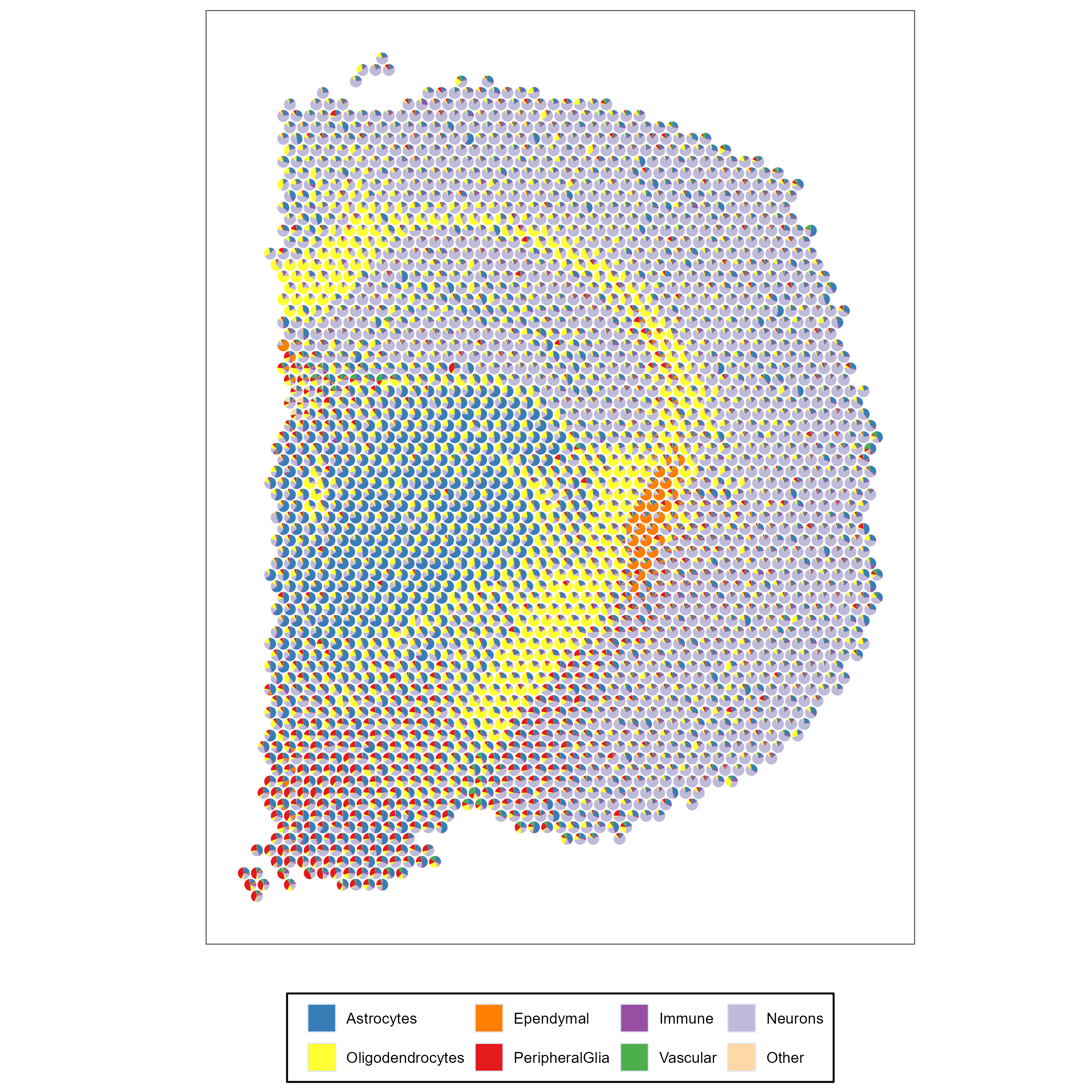

To make a scatterheatmap showing the predicted proportions for a selected cell type:

SMART_scatterheatmap(visium_mouse_brain$loc,res$ct_proportions, celltype = 'Oligos')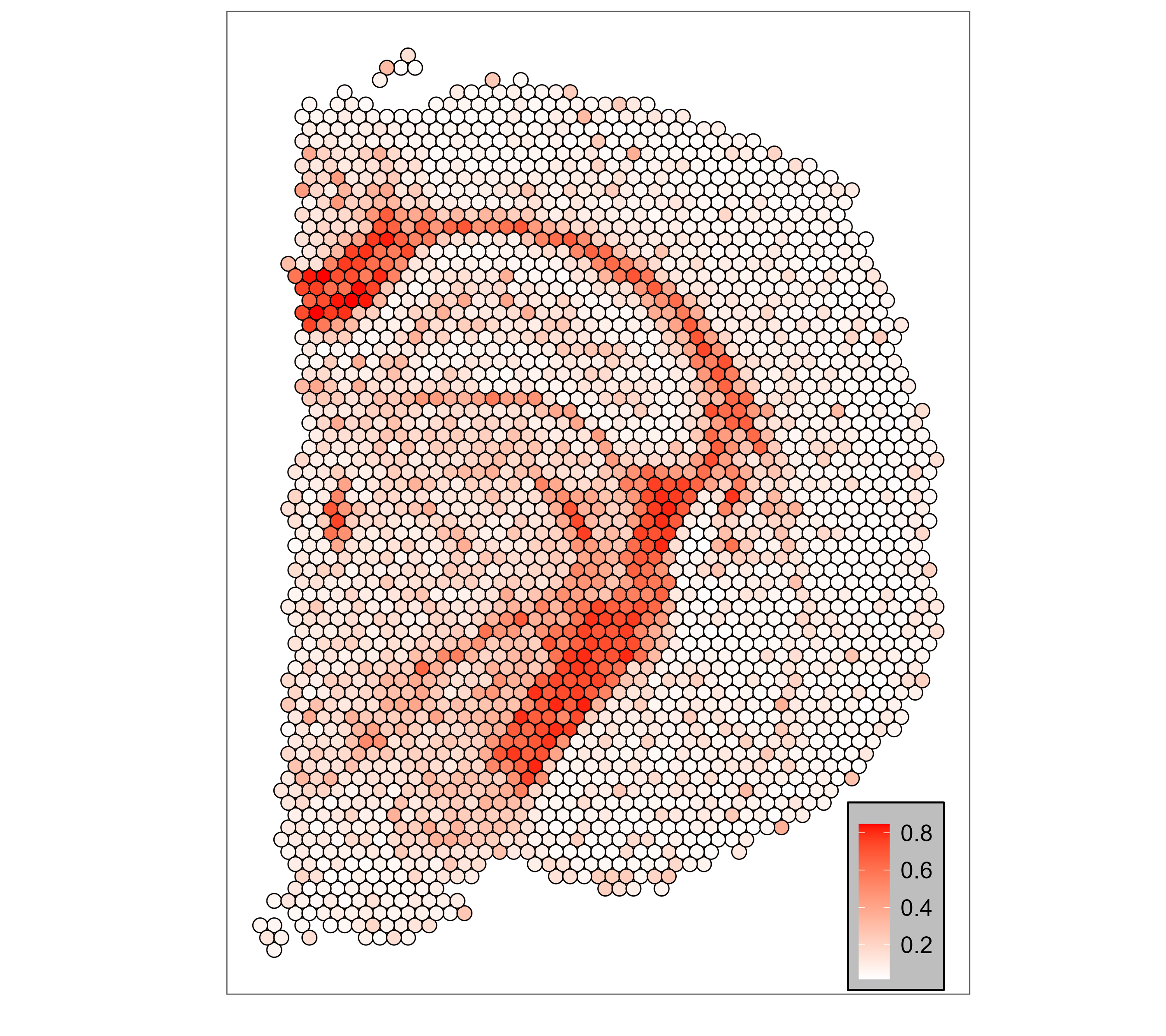

The covariate model of SMART takes the spatial transcriptomics data matrix (stData), a list of marker gene symbols for each cell type (markerGs), a data.frame of covariate levels (covarDat) and the covariates (covars) as inputs.

Run the covariate model with:

data(MPOA)
mod <- SMART_covariate(stData=MPOA$stMat, markerGs=MPOA$markers,       
                       covarDat=MPOA$covDat,covars='sex',
                       noMarkerCts=1,outDir='SMART_results', seed=1)
cov_res <- get_est(model=mod$model, stData=MPOA$stMat, 
                   covarDat=MPOA$covDat, covar='sex')

Then, we can compute the log2 fold change between the conditions (Female vs. Male).

geneList=log2(cov_res$ct_spec_gexp$F$phi/cov_res$ct_spec_gexp$M$phi)['Inhibitory',] %>% sort()

Next, we perform a gene set enrichment analysis for each cell type. Here we use the "fgsea" R package to obtain the GO biological processes, GO molecular functions, and Reactome pathways associated with sex. The .gmt files can be downloaded from MSigDB (https://www.gsea-msigdb.org/gsea/msigdb/index.jsp).

library(fgsea)
gseaRes=list()
for(gmt in c('m5.go.bp.v2023.1.Mm.symbols.gmt','m5.go.mf.v2023.1.Mm.symbols.gmt',
             'm2.cp.reactome.v2023.1.Mm.symbols.gmt')){
		print(gmt)
		pathways <- gmtPathways(paste0('GSEA/',gmt))
		fgseaRes <- fgsea(pathways = pathways,
						stats    = geneList,
						minSize  = 10,
						maxSize  = 1000,
						nperm=1000)
		gseaRes[[gmt]]=fgseaRes %>% filter(padj<0.1) %>% arrange(pval) %>% mutate(database=gmt)
}	
gseaRes=rbindlist(gseaRes)

The two-stage model of SMART takes the spatial transcriptomics data matrix (stData), a list of marker gene symbols to be used to deconvolve cell types into major cell types (markers_S1), a list of marker gene symbols to be used to deconvolve the cell type of interest into its subtypes (markers_S2), the cell type of interest (CT_OI), the cell type that is transcriptomically similar to the cell type of interest (CT_similar) as inputs.

The CT_similar can be NULL, a character value specifying a cell type name, or 'auto' to automatically select the most similar cell type.

Run the two-stage model with:

data(NSCLC)
TS_res <- SMART_2S(NSCLC$stData, NSCLC$markers_S1, NSCLC$markers_S2,
                   noMarkerCts_S1=1, noMarkerCts_S2=1,
                   CT_OI='DC',CT_similar='macrophage',
                   outDir='SMART_results')

The resulting object contains the models from each of the two stages as well as the final cell type proportions of each spot.