Mataveid is a basic system identification toolbox for both GNU Octave and MATLAB®. Mataveid is based on the power of linear algebra and the library is easy to use. Mataveid using the classical realization and polynomal theories to identify state space models from data. There are lots of subspace methods in the "old" folder and the reason why I'm not using these files is because they can't handle noise quite well.
I'm building this library because I feel that the commercial libraries are just for theoretical experiments. I'm focusing on real practice and solving real world problems.
| Function | Status | Comment |
|---|---|---|
rpca.m |
Complete | Nothing to do here |
filtfilt.m |
Complete | Nothing to do here |
pf.m |
Complete | Nothing to do here |
spa.m |
Complete | Nothing to do here |
arx.m |
Complete | Nothing to do here |
oe.m |
Complete | Nothing to do here |
armax.m |
Complete | Nothing to do here |
cca.m |
Almost complete | Returns kalman gain matrix K, need to have a practical example |
rls.m |
Almost complete | Returns kalman gain matrix K, need to have a better practical example |
eradc.m |
Almost complete | Added a kalman filter, need to have a pratical example |
n4sid.m |
Almost complete | Added a kalman filter, need to have a better pratical example |
moesp.m |
Almost complete | Added a kalman filter, need to have a pratical example |
sra.m |
Almost complete | Upload measurement sensor system |
bj.m |
Almost complete | Find a pratical example |
sindy.m |
Ongoing | Easier to use, return jacobian model for linearization |
ocid.m |
Ongoing | Find a pratical example and test it, test the observer with ocid.m |
sr_ukf_parameter_estimation.m |
Ongoing | Find a practical example for a hydraulic orifice |
sr_ukf_state_estimation.m |
Ongoing | Use with sindy.m and a pratical example |
ortjiop.m |
Ongoing | Find a practical example |
idbode.m |
Ongoing | Find a practical example |
ica.m |
Ongoing | Find a practical example |
svm.m |
Ongoing | Find a practical example with image classification and PCA |
okid.m |
Not created yet | Create the okid.m file and make sure it is robust against noise and also returns K matrix. Borrow code from the old folder. |
Installing GNU Octave's Control-Toolbox or MATLAB's Control-Toolbox/System Identification Toolbox will cause problems with MataveID & MataveControl because they are using the same function names.
- ERA-DC for mechanical damped systems in the time plane
- SINDY for multivariable abritary nonlinear systems
- RLS for all kind of arbitary single input and single output systems
- OCID for closed loop identification, observer identification and controller identification
- ORTJIOP for stochastic closed loop, plant and controller identification
- FILTFILT for low pass filtering without phase delay
- SPA for spectral analysis
- IDBODE for mechanical damped systems in the frequency plane
- RPCA for filtering data and images
- ICA for separating signals so they are independent from each other
- SR-UKF-Parameter-Estimation for finding parameters from an very complex system of equation if data is available
- SR-UKF-State-Estimation for filtering noise and estimate the state of a system
- SVM for C-code classification of data for CControl
- N4SID for regular linear state space systems
- MOESP for regular linear state space systems
- CCA for linear stochastic state space systems
- SRA for stochastic model identification
- PF for particle filter for non-gaussian state estimation filtering
- BJ for estimate system model and disturbance model
Mataveid contains realization identification, polynomal algorithms and subspace algorithms. They can be quite hard to understand, so I highly recommend to read papers in the "reports" folder about the algorithms if you want to understand how they work, or read the literature.
I have been using these books for creating the .m files. All these books have different audience. Some techniques are meant for researchers and some are meant for practical engineering.
This book include techniques for linear mechanical systems such as vibrating beams, damping, structural mechanics etc. These techniques comes from NASA and the techniques are created by Jer-Nan Juang. This is a very practical book. The book uses the so called realization theory methods for identify dynamical models from data.
Advantages:
- Easy to read and very practical
- Include mechanical model buildning
- Include impulse, frequency, stochastic, closed loop and recursive identification
- These techniques are applied onto Hubble Telescope, Space Shuttle Discovery and Galileo spacecraft
Disadvantages:
- Do not include nonlinear system identification and subspace methods
- Do not include filtering
- MATLAB files from this book is export controlled from NASA = Difficult to download
- This book is not produced anymore. I have the PDF.

This book covering techniques for all types of systems, linear and nonlinear, but it's more a general book for system identfication. Professor Rolf Johansson book contains lots of practice, but also theory as well. More theory and less practice compared to Applied System Identification from Jer-Nan Juang. This book uses both the realization theory methods and subspace methods for identify dynamical systems from data. Also this book includes filters as well such as Uncented Kalman Filter. Can be purchased from https://kfsab.se/sortiment/system-modeling-and-identification/
Advantages:
- Easy to read and somtimes practical
- Include filtering, statistics and other types of modeling techniques
- Include impulse, frequency, stochastic, closed loop, nonlinear and recursive identification
- Include both realization theory, subspace and nonlinear system identification methods
Disadvantages:
- Do not include closed loop identification
- Some methods are difficult to understand how to apply with MATLAB-code. Typical univerity literature for students
This book include techniques for all types of linear systems. It's a general book of linear system identification. The advantages of this book is that it include modern system identification techniques. The disadvantages about this book is that it contains only theory and no practice, but Professor Tohru Katayama, have made a great work for collecting all these subspace methods. Use this book if you want to have knowledge about the best subspace identification methods.
Advantages:
- Include MATLAB code examples and lots of step by step examples
- Include stochastic and closed identification
- Include the latest methods for linear system identification
- Include both realization theory and subspace system identification methods
Disadvantages:
- Difficult to read and understand
- Does not include impulse, frequency and nonlinear identification
- Does not include filtering, statistics and other types of modeling techniques

This book is only for adaptive control. But there is one algorithm that are very useful - Recursive Least Squares. This is a very pratical book for applied adaptive control. It's uses the legacy SISO adaptive techniques such as pole placement, Self Tuning Regulator(STR) and Model Reference Adaptive Systems(MRAS) combined with Recursive Least Squares(RLS). If you wonder why only SISO and not MIMO, it's because adaptive control is very difficult to apply in practice and create a reliable controller for all types of systems. The more difficult problem is to solve, the more simplier technique need to be used.
Advantages:
- The authors of the book explains which chapters are for pratcial engineering and theoretical researchers
- Easy to read
- Include both advanced and simple methods depending on which type of problem to solve
Disadvantages:
- Only one system identification algorithm is taught
- Only SISO model are applied
- This book is made for adaptive control and have only one chapter that contains system identification
MOESP is an algorithm that identify a linear state space model. It was invented in 1992. It can both identify SISO and MISO models. Try MOESP or N4SID. They give the same result, but sometimes MOESP can be better than N4SID. It all depends on the data.
[sysd] = moesp(u, y, k, sampleTime, delay, systemorder); % k = Integer tuning parameter such as 10, 20, 25, 32, 47 etc.clc; clear close all;
[u, t] = gensig('square', 10, 10, 100);
G = tf(1, [1 0.8 3]); % Model
y = lsim(G, u, t); % Simulation
y = y + 0.4*rand(1, length(t));
close
k = 30;
sampleTime = t(2) - t(1);
systemorder = 3;
delay = 0;
ktune = 0.01;
[sysd, K] = moesp(u, y, k, sampleTime, ktune, delay, systemorder); % This example works better with MOESP, rather than N4SID
% Create the observer
observer = ss(sysd.delay, sysd.A - K*sysd.C, [sysd.B K], sysd.C, [sysd.D sysd.D*0]);
observer.sampleTime = sysd.sampleTime;
% Check observer
[yf, tf] = lsim(observer, [u; y], t);
close
plot(tf, yf, t, y)
grid on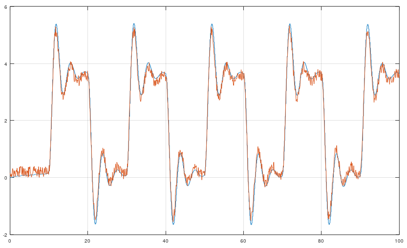
N4SID is an algoritm that identify a linear state space model. Use this if you got regular data from a dynamical system. This algorithm can handle both SISO and MISO. N4SID algorithm was invented 1994. If you need a nonlinear state space model, check out the SINDy algorithm. Try N4SID or MOESP. They give the same result, but sometimes N4SID can be better than MOESP. It all depends on the data.
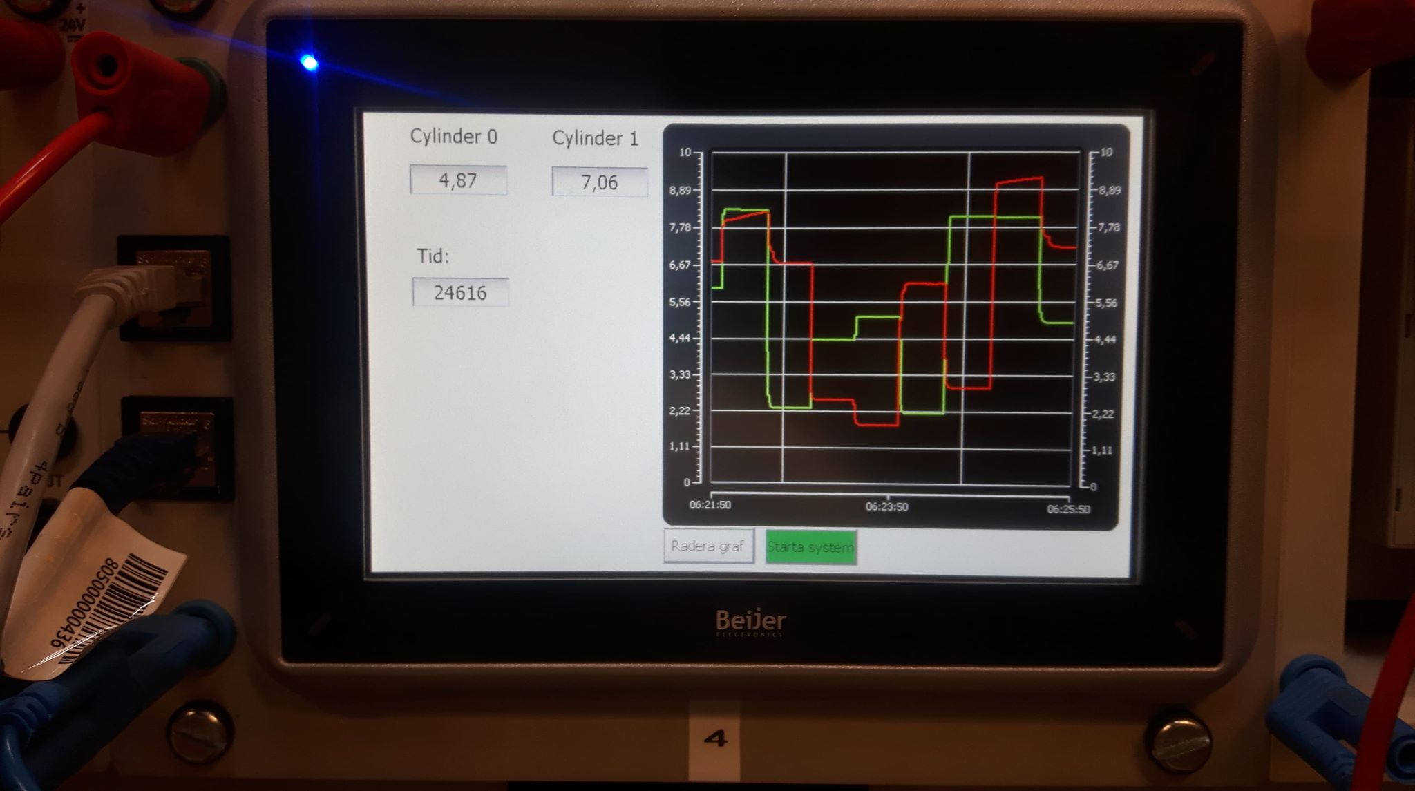
[sysd, K] = n4sid(u, y, k, sampleTime, ktune, delay, systemorder); % k = Integer tuning parameter such as 10, 20, 25, 32, 47 etc. ktune = kalman filter tuning such as 0.1, 0.01 etcHere I programmed a Beijer PLC that controls the multivariable cylinder system. It's a nonlinear system, but N4SID can handle it because it's not so nonlinear as a hydraulic motor. Cylinder 0 and Cylinder 1 affecting each other when the propotional control valves opens.
clc; clear; close all;
% Load the data
X = csvread('..\data\MultivariableCylinders.csv');
t = X(:, 1);
r0 = X(:, 2);
r1 = X(:, 3);
y0 = X(:, 4);
y1 = X(:, 5);
sampleTime = 0.1;

% Transpose the CSV data
u = [r0';r1'];
y = [y0';y1'];
t = t';

% Create the model
k = 10;
sampleTime = t(2) - t(1);
ktune = 0.01; % Kalman filter tuning
% This won't result well with MOESP and system order = 2
[sysd, K] = n4sid(u, y, k, sampleTime, ktune); % Delay argment is default 0. Select model order = 2 when n4sid ask you

% Create the observer
observer = ss(sysd.delay, sysd.A - K*sysd.C, [sysd.B K], sysd.C, [sysd.D sysd.D*0]);
observer.sampleTime = sysd.sampleTime;

% Do simulation
[outputs, T, x] = lsim(observer, [u; y], t);
close
plot(T, outputs(1, :), t, y(1, :))
title('Cylinder 0');
xlabel('Time');
ylabel('Position');
grid on
legend('Identified', 'Measured');
ylim([0 12]);
figure
plot(T, outputs(2, :), t, y(2, :))
title('Cylinder 1');
xlabel('Time');
ylabel('Position');
grid on
legend('Identified', 'Measured');
ylim([0 12]);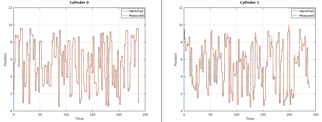
If N4SID won't work for you due to high noise measurement, then CCA is an alternative method to use. CCA returns a state space model and a kalman gain matrix K.
[sysd, K] = cca(u, y, k, sampleTime, delay); % k = Integer tuning parameter such as 10, 20, 25, 32, 47 etc.clc; clear; close all;
% Create model
G = tf(1, [1 1.5 1]);
% Create control inputs
[u, t] = gensig('square', 10, 10, 100);
u = [u*5 u*2 -u 10*u -2*u];
t = linspace(0, 50, length(u));
% Simulate
y = lsim(G, u, t);
close
% Add noise
yn = y + randn(1, length(y));
% Identify the model
sampleTime = t(2) - t(1);
delay = 0;
systemOrder = 2;
k = 30;
[sysd, K] = cca(u, yn, k, sampleTime, delay, systemOrder);
% Create an observer
delay = sysd.delay;
A = sysd.A;
B = sysd.B;
C = sysd.C;
D = sysd.D;
observer = ss(delay, A - K*C, [B K], C, [D 0]);
observer.sampleTime = sysd.sampleTime;
% Simulate the observer
[yobs, tobs] = lsim(observer, [u; yn], t);
close
plot(t, yn, '-r', tobs, yobs, '-b');
grid on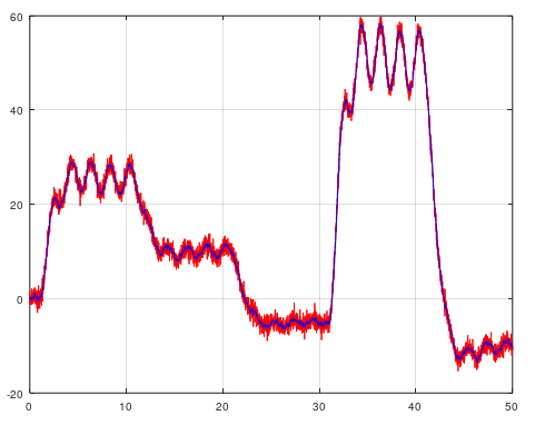
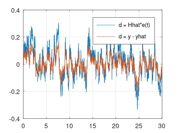
This is an algorithm that can identify a stochastic model from error measurement data.
[sysd, K] = sra(e, k, sampleTime, ktune, delay, systemorder);% Clear all
clear all
% Create system model
G = tf(1, [1 1.5 2]);
% Create disturbance model
H = tf([2 3], [1 5 6]);
% Create input signal
[u, t] = gensig('square', 10, 10, 100);
u = [u*5 u*2 -u 10*u -2*u];
t = linspace(0, 30, length(u));
% Create disturbance signal
e = randn(1, length(t));
% Simulate with noise-
y = lsim(G, u, t) + lsim(H, e, t);
close
% Identify a system model
k = 50;
sampleTime = t(2) - t(1);
delay = 0;
systemorder = 2;
Ghat = cca(u, y, k, sampleTime, delay, systemorder);
% Find the disturbance d = H*e
Ad = Ghat.A;
Bd = Ghat.B;
Cd = Ghat.C;
Dd = Ghat.D;
x = zeros(systemorder, 1);
for i = 1:size(t, 2)
yhat(:,i) = Cd*x + Dd*u(:,i);
x = Ad*x + Bd*u(:,i); % Update state vector
end
d = y - yhat;
% Identify the disturbance model
systemorder = 2;
ktune = 0.5;
[Hhat] = sra(d, k, sampleTime, ktune, delay, systemorder);
% Simulate the disturbance model
[dy, dt] = lsim(Hhat, e, t);
close
plot(dt, dy, t, d);
legend('d = Hhat*e(t)', 'd = y - yhat')
grid on
% Clear all
clear all

% Create disturbance signal
t = linspace(0, 100, 1000);
e = randn(1, length(t));

% Create disturbance model
H = tf([1], [1 3]);

% Simulate
y = lsim(H, e, t);
close

% Identify a model
k = 100;
sampleTime = t(2) - t(1);
ktune = 0.01;
delay = 0;
systemorder = 2;
[H, K] = sra(y, k, sampleTime, ktune, delay, systemorder);

% Observer
H.A = H.A - K*H.C;

% Create new signals
[y, t] = gensig('square', 10, 10, 100);
y = [y*5 y*2 -y 10*y -2*y];
t = linspace(0, 100, length(y));

% Add some noise
y = y + 2*randn(1, length(y));

% Simulate
lsim(H, y, t);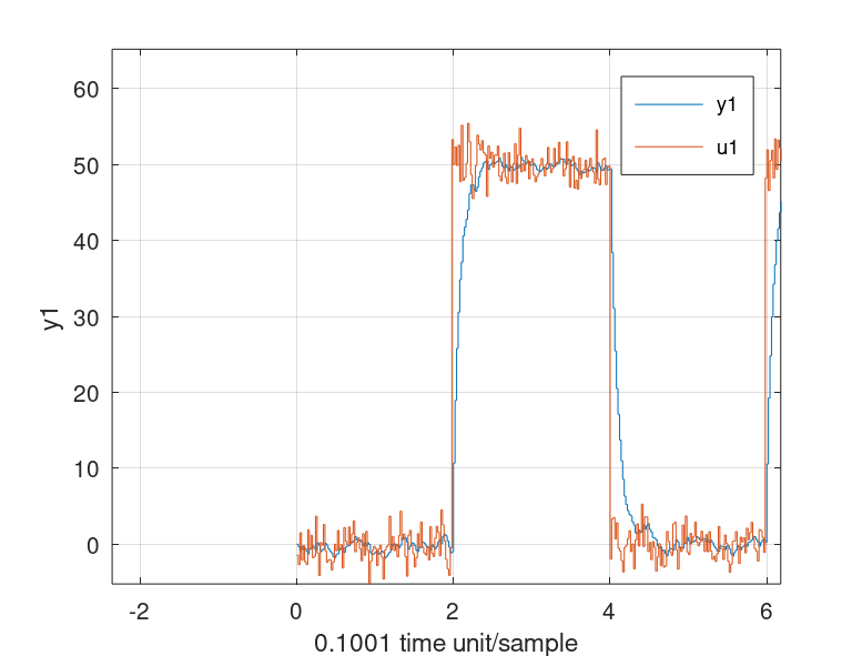
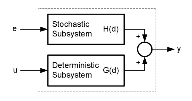
Box-Jenkins is a special case when a system model sysd and a disturbance model sysh need to be found. The disturbance is difficult to know and with this Box-Jenkins algorithm, then the user can identify the disturbance model and create an observer of it by using the kalman gain matrices K1, K2. Notice that this Box-Jenkins algorithm using subspace methods, instead of classical polynomial methods.
The disturbance model can be used for:
- Create a disturbance simulation with feedback control
- Create filtering for sensors
[sysd, K1, sysh, K2] = bj(u, y, k, sampleTime, ktune, delay, systemorder_sysd, systemorder_sysh);% Clear all
clear all
close all
% Create system model
G = tf(1, [1 1.5 2]);
% Create disturbance model
H = tf([2 3], [1 5 6]);
% Create input signal
[u, t] = gensig('square', 10, 10, 100);
u = [u*5 u*2 -u 10*u -2*u];
t = linspace(0, 30, length(u));
% Create disturbance signal
e = randn(1, length(t));
% Simulate with noise
d = lsim(H, e, t);
y = lsim(G, u, t) + d
close
% Use Box-Jenkins to find the system model and the disturbance model
k = 50;
sampleTime = t(2) - t(1);
ktune = 0.5;
delay = 0;
systemorder_sysd = 2;
systemorder_sysh = 2;
[sysd, K1, sysh, K2] = bj(u, y, k, sampleTime, ktune, delay, systemorder_sysd, systemorder_sysh);
% Plot sysd
[sysd_y, sysd_t] = lsim(sysd, u, t);
close all
plot(t, y, sysd_t, sysd_y);
legend('Measurement', 'Identified')
grid on
title('System model', 'FontSize', 20)
% Plot sysh
figure(2)
[sysh_y, sysh_t] = lsim(sysh, e, t);
close(2)
figure(2)
plot(t, d, sysh_t, sysh_y);
legend('Measurement', 'Identified')
grid on
title('Disturbance model', 'FontSize', 20)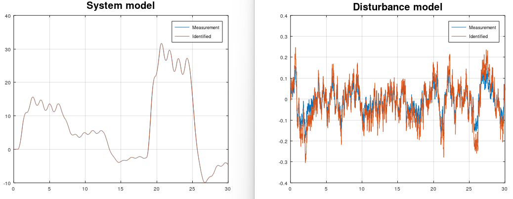
RLS is an algorithm that creates a SISO model from data. Here you can select if you want to estimate an ARX, OE model or an ARMAX model, depending on the number of zeros in the polynomal "nze". Select number of error-zeros-polynomal "nze" to 1, and you will get a ARX model or select "nze" equal to model poles "np", you will get an ARMAX model that also includes a kalman gain matrix K. I recommending that. This algorithm can handle data with noise. This algorithm was invented 1821 by Carl Friedrich Gauss, but it was until 1950 when it got its attention in adaptive control.
Use this algorithm if you have data from a open/close loop system and you want to apply that algorithm into embedded system that have low RAM and low flash memory. RLS is very suitable for system that have a lack of memory.
There is a equivalent C-code for RLS algorithm here. Works on ALL embedded systems. https://github.com/DanielMartensson/CControl
[sysd, K] = rls(u, y, np, nz, nze, sampleTime, delay, forgetting);Notice that there are sevral functions that simplify the use of rls.m
[sysd, K] = oe(u, y, np, nz, sampleTime, delay, forgetting);
[sysd, K] = arx(u, y, np, nz, sampleTime, ktune, delay, forgetting);
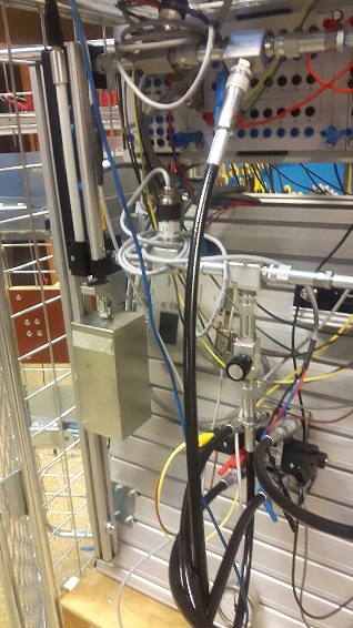
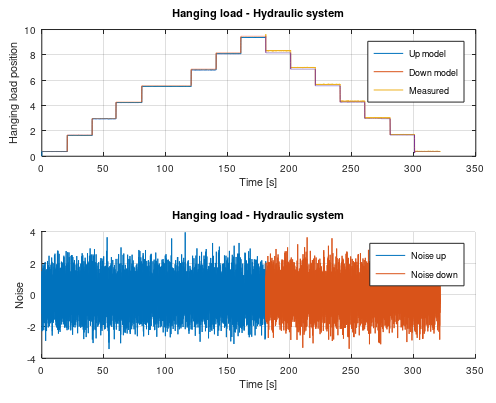
[sysd, K] = armax(u, y, np, nz, nze, sampleTime, ktune, delay, forgetting);This is a hanging load of a hydraulic system. This system is a linear system due to the hydraulic cylinder that lift the load. Here I create two linear first order models. One for up lifting up and one for lowering down the weight. I'm also but a small orifice between the outlet and inlet of the hydraulic cylinder. That's create a more smooth behavior. Notice that this RLS algorithm also computes a Kalman gain matrix.
% Load data
X = csvread('..\data\HangingLoad.csv');
t = X(:, 1)'; % Time
r = X(:, 2)'; % Reference
y = X(:, 3)'; % Output position
u = X(:, 4)'; % Input signal from P-controller with gain 3
sampleTime = 0.02;

% Do identification of the first data set
l = length(r) + 2000; % This is half data

% Poles and zeros
np = 1; % Number of poles for A(q)
nz = 1; % Number of zeros of B(q)
nze = 1; % Number of zeros of C(q)

% Model up
u_up = r(1:l/2);
e_up = randn(1, length(u_up)); % Noise
y_up = y(1:l/2) + e_up;
[sysd, K] = rls(u_up, y_up, np, nz, nze, sampleTime);

% Observer
sysd_up = ss(0, sysd.A - K*sysd.C, [sysd.B K], sysd.C, [sysd.D 0]);
sysd_up.sampleTime = sysd.sampleTime;

% Model down
u_down = r(l/2+1:end);
e_down = randn(1, length(u_down)); % Noise
y_down = y(l/2+1:end) + e_down;
[sysd, K] = rls(u_down, y_down, np, nz, nze, sampleTime);

% Observer
sysd_down = ss(0, sysd.A - K*sysd.C, [sysd.B K], sysd.C, [sysd.D 0]);
sysd_down.sampleTime = sysd.sampleTime;

% Simulate model up
time_up = t(1:l/2);
[~,~,x] = lsim(sysd_up, [u_up; e_up], time_up);
hold on

% Simulate model down
time_down = t(l/2+1:end);
x0 = x(:, end); % Initial state
lsim(sysd_down, [u_down; e_down], time_down, x0);

% Place legend, title, labels for the signals
subplot(2, 1, 1)
legend('Up model', 'Down model', 'Measured');
title('Hanging load - Hydraulic system')
xlabel('Time [s]')
ylabel('Hanging load position');

% Place legend, title, labels for the noise
subplot(2, 1, 2)
legend('Noise up', 'Noise down');
title('Hanging load - Hydraulic system')
xlabel('Time [s]')
ylabel('Noise');
Here we can se that the first model follows the measured position perfect. The "down-curve" should be measured a little bit longer to get a perfect linear model.
ERA/DC was invented 1987 and is a successor from ERA, that was invented 1985 at NASA. The difference between ERA/DC and ERA is that ERA/DC can handle noise much better than ERA. But both algorihtm works as the same. ERA/DC want an impulse response. e.g called markov parameters. You will get a state space model from this algorithm. This algorithm can handle both SISO and MISO data.
Use this algorithm if you got impulse data from e.g structural mechanics.
[sysd, K] = eradc(g, sampleTime, ktune, delay systemorder);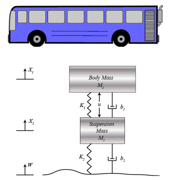
clc; clear; close all

%% Parameters
m1 = 2.3;
m2 = 3.1;
k1 = 8.5;
k2 = 5.1;
b1 = 3.3;
b2 = 5.1;

A=[0                 1   0                                              0
  -(b1*b2)/(m1*m2)   0   ((b1/m1)*((b1/m1)+(b1/m2)+(b2/m2)))-(k1/m1)   -(b1/m1)
   b2/m2             0  -((b1/m1)+(b1/m2)+(b2/m2))                      1
   k2/m2             0  -((k1/m1)+(k1/m2)+(k2/m2))                      0];
B=[0 0;
   1/m1 0;
   0 0 ;
   (1/m1)+(1/m2) 1/m2];
C=[0 0 1 0;
   0 1 0 0];
D=[0 0;
   0 0];
delay = 0;

%% Model
buss = ss(delay,A,B,C,D);

%% Simulation
[g, t] = impulse(buss, 10);

% Reconstruct the input impulse signal from impulse.m
u = zeros(size(g));
u(1) = 1;

%% Add 15% noise
v = 2*randn(1, 1000);
for i = 1:length(g)-1
  noiseSigma = 0.15*g(i);
  noise = noiseSigma*v(i); % v = noise, 1000 samples -1 to 1
  g(i) = g(i) + noise;
end

%% Identification
systemorder = 10;
ktune = 0.09;
sampleTime = t(2) - t(1);
delay = 0;
[sysd, K] = eradc(g, sampleTime, ktune, delay systemorder);

% Create the observer
observer = ss(sysd.delay, sysd.A - K*sysd.C, [sysd.B K], sysd.C, [sysd.D sysd.D*0]);
observer.sampleTime = sysd.sampleTime;

%% Validation
[gf, tf] = lsim(observer, [u; g], t);
close

%% Check
plot(t, g, tf, gf)
legend('Data 1', 'Data 2', 'Identified 1', 'Identified 2', 'location', 'northwest')
grid on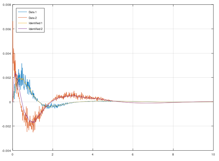
This is an extention from OKID. The idea is the same, but OCID creates a LQR contol law as well. This algorithm works only for closed loop data. It have its orgin from NASA around 1992 when NASA wanted to identify a observer, model and a LQR control law from closed loop data that comes from an actively controlled aircraft wing in a wind tunnel at NASA Langley Research Center. This algorithm works for both SISO and MIMO models.
Use this algorithm if you want to extract a LQR control law, kalman observer and model from a running dynamical system. Or if your open loop system is unstable and it requries some kind of feedback to stabilize it. Then OCID is the perfect choice.
This OCID algorithm have a particle filter that estimates the markov parameters.
[sysd, K, L] = ocid(r, uf, y, sampleTime, alpha, regularization, systemorder);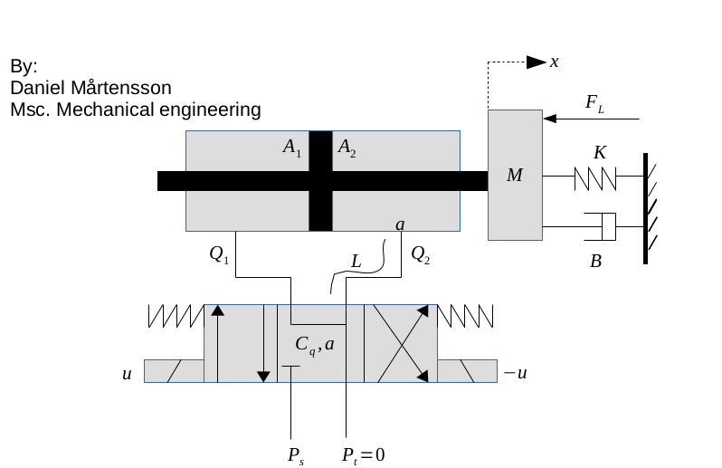
%% Matrix A
A = [0 1  0  0;
    -7 -5 0  1;
     0 0  0  1;
     0 1 -8 -5];

%% Matrix B
B = [0 0;
     1 0;
     0 0;
     0 1];

%% Matrix C
C = [1 0 0 0;
     0 0 0 1];

%% Model and signals
delay = 0;
sys = ss(delay, A, B, C);
t = linspace(0, 20, 1000);
r = [linspace(5, -11, 100) linspace(7, 3, 100) linspace(-6, 9, 100) linspace(-7, 1, 100) linspace(2, 0, 100) linspace(6, -9, 100) linspace(4, 1, 100) linspace(0, 0, 100) linspace(10, 17, 100) linspace(-30, 0, 100)];
r = [r;2*r]; % MIMO

%% Feedback
Q = sys.C'*sys.C;
R = [1 0; 0 1];
L = lqr(sys, Q, R);
[feedbacksys] = reg(sys, L);
yf = lsim(feedbacksys, r, t);
close

%% Add noise
v = 2*randn(1, 1000);
for i = 1:length(yf)
  noiseSigma = 0.10*yf(:, i);
  noise = noiseSigma*v(i); % v = noise, 1000 samples -1 to 1
  yf(:, i) = yf(:, i) + noise;
end

%% Identification
uf = yf(3:4, :); % Input feedback signals
y = yf(1:2, :); % Output feedback signals
regularization = 10000;
modelorder = 6;
sampleTime = t(2) - t(1);
alpha = 20; % Filtering integer parameter
[sysd, K, L] = ocid(r, uf, y, sampleTime, alpha, regularization, modelorder);

%% Validation
u = -uf + r; % Input signal %u = -Lx + r = -uf + r
yt = lsim(sysd, u, t);
close

%% Check
plot(t, yt(1:2, 1:2:end), t, yf(1:2, :))
legend("Identified 1", "Identified 2", "Data 1", "Data 2", 'location', 'northwest')
grid on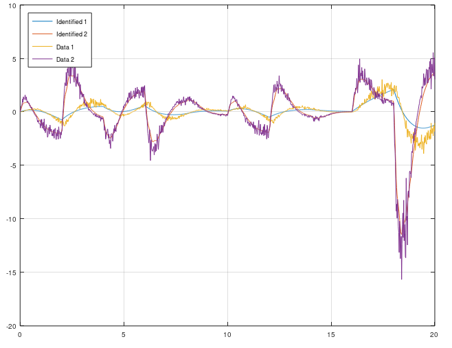
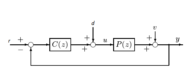
This algorithm identify the closed loop system, plant and controller. The difference between OCID and Orthogonal Decomposition of Joint Input-Output Process (ORTJIOP) is that OCID identifies the plant model, LQR control law and kalman gain matrix. The ORTJIOP identifies the closed loop system, plant model and controller. But not LQR controller. Instead, ORTJIOP returns the controller as it was a dynamical model. ORTJIOP can have disturbance onto the input system of the plant as well.
[sysd, P, C] = ortjiop(u, y, r, d, k, sampleTime, delay, systemorder);% Will upload soon a practical example with real measurementsThis is a new identification technique made by Eurika Kaiser from University of Washington. It extends the identification methods of grey-box modeling to a much simplier way. This is a very easy to use method, but still powerful because it use least squares with sequentially thresholded least squares procedure. I have made it much simpler because now it also creates the formula for the system. In more practical words, this method identify a nonlinear ordinary differential equations from time domain data.
This is very usefull if you have heavy nonlinear systems such as a hydraulic orifice or a hanging load.
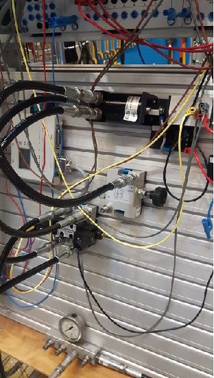
This example is a real world example with noise and nonlinearities. Here I set up a hydraulic motor in a test bench and measure it's output and the current to the valve that gives the motor oil. The motor have two nonlinearities - Hysteresis and the input signal is not propotional to the output signal. By using two nonlinear models, we can avoid the hysteresis.
% Load CSV data
X = csvread('MotorRotation.csv'); % Can be found in the folder "data"
t = X(:, 1);
u = X(:, 2);
y = X(:, 3);
sampleTime = 0.02;

% Do filtering of y
y = filtfilt2(y', t', 0.1)';

% Sindy - Sparce identification Dynamics
activations = [1 1 1 1 1 1 1 1 1 0 0 0 0 0 0 0 0 0 0 0 0 0 0 0 0 0 0 0 0 0 0 0 0 0 0 0 0 0 0 0 0 0 0 0 0 0 0 0 0 0 0]; % Enable or disable the candidate functions such as sin(u), x^2, sqrt(y) etc...
lambda = 0.05;
l = length(u);
h = floor(l/2);
s = ceil(l/2);
fx_up = sindy(u(1:h), y(1:h), activations, lambda, sampleTime); % We go up
fx_down = sindy(u(s:end), y(s:end), activations, lambda, sampleTime); % We go down

% Simulation up
x0 = y(1:h)(1);
u_up = u(1:h)(1:100:end)';
stepTime = 1.2;
[x_up, t] = nlsim(fx_up, u_up, x0, stepTime, 'ode15s');

% Simulation down
x0 = y(s:end)(1);
u_down = u(s:end)(1:100:end)';
stepTime = 1.2;
[x_down, t] = nlsim(fx_down, u_down, x0, stepTime, 'ode15s');

% Compare
close all
plot([x_up x_down])
hold on
plot(y(1:100:end));
legend('Simulation', 'Measurement')
ylabel('Rotation')
xlabel('Time')
grid on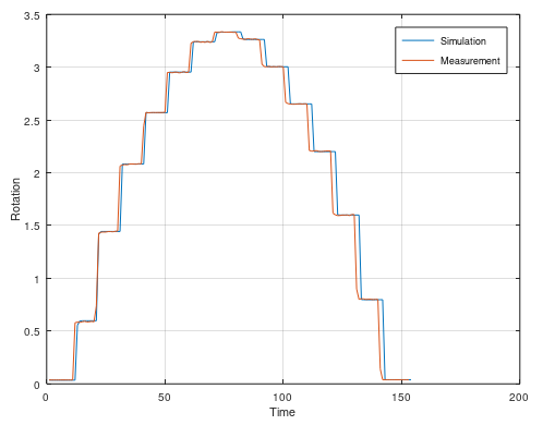
Here is a multivariable example with SINDy. It use the same data as the OKID scenario.
% Data
X = csvread('MultivariableCylinders.csv');
t = X(:, 1);
r0 = X(:, 2); % Reference 0
r1 = X(:, 3); % Reference 1
y0 = X(:, 4); % Output 0
y1 = X(:, 5); % Output 1
sampleTime = 0.1;

% Identification
inputs = [r0 r1];
outputs = [y0 y1];
activations = [1 1 1 1 1 1 1 1 1 1 1 1 1 1 1 1 1 1 1 1 1 1 1 1 1 1 1 1 1 1 1 1 1 1 1 1 1 1 1 1 1 1 1 1 1 1 1 1 1 1 1 1 1 1 1 1 1 1 1 1 1 1 1 1 1 1 1 1 1 1 1 1 1 1 1 1 1 1 1 1 1 1 1 1 1 1 1 1 1 1 1 1 1 1 1 1 1 1 0 0 0 0 0 0 0 0 0 0 0 0 0 0 0 0 0 0 0 0 0 0 0 0 0 0 0];
lambda = 0.2;
model = sindy(inputs, outputs, activations, lambda, sampleTime);

% Simulation
u = inputs';
x0 = outputs'(:, 1);
stepTime = 1.0;
[x, t] = nlsim(model, u, x0, stepTime, 'ode15s');

% Compare
close all
plot(x(1, :))
hold on
plot(y0)
legend('Simulation', 'Measurement')
ylabel('Position')
xlabel('Time')
title('Cylinder 0')
grid on

figure
plot(x(2, :))
hold on
plot(y1)
legend('Simulation', 'Measurement')
ylabel('Position')
xlabel('Time')
title('Cylinder 1')
grid on
This plots a bode diagram from measurement data. It can be very interesting to see how the amplitudes between input and output behaves over frequencies. This can be used to confirm if your estimated model is good or bad by using the bode command from Matavecontrol and compare it with idebode.
idbode(u, y, w);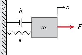
%% Model of a mass spring damper system
M = 5; % Kg
K = 100; % Nm/m
b = 52; % Nm/s^2
G = tf([1], [M b K]);

%% Frequency response
t = linspace(0, 50, 3000);
[u, fs] = chirp(t);

%% Simulation
y = lsim(G, u, t);
close all

% Add noise
y = y + 0.0001*randn(1, length(y));

%% Identify bode diagram
idbode(u, y, fs);

%% Check
bode(G);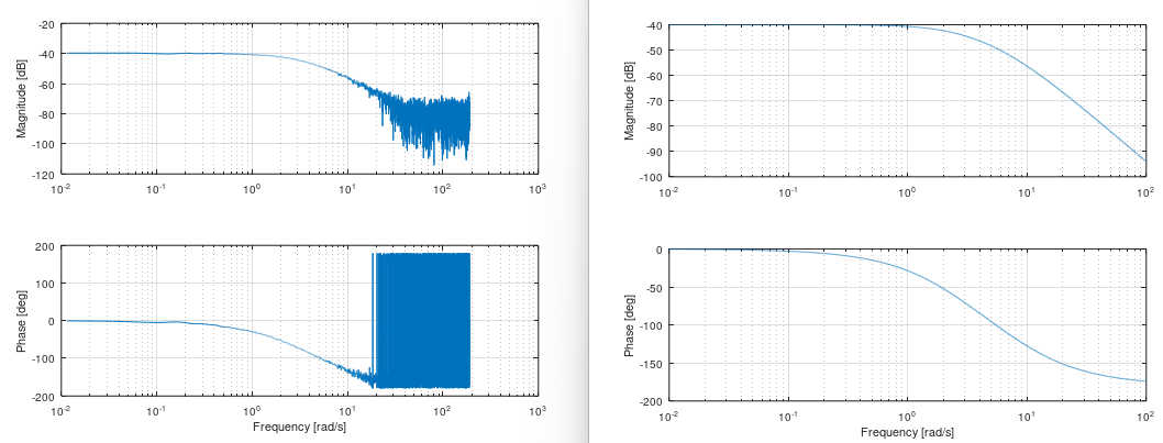
This plots all the amplitudes from noisy data over its frequencies. Very good to see what type of noise or signals you have. With this, you can determine what the real frequencies and amplitudes are and therefore you can create your filtered frequency response that are clean.
[amp, wout] = spa(y, t);Assume that we are using the previous example with different parameters.
%% Frequency input
t = linspace(0.0, 100, 30000);
u1 = 2*sin(2*pi*5.*t); % 5 Hz
u2 = 6*sin(2*pi*10.*t); % 10 Hz
u3 = 10*sin(2*pi*20.*t); % 20 Hz
u4 = 20*sin(2*pi*8.*t); % 8 Hz
u = u1 + u2 + u3 + u4;

%% Noise
u = u + 5*randn(1, 30000);

%% Identify what frequencies and amplitudes we had!
spa(u, t);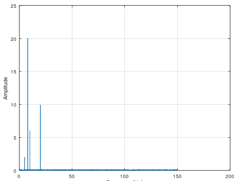
This filter away noise with a good old low pass filter that are being runned twice. Filtfilt is equal to the famous function filtfilt in MATLAB, but this is a regular .m file and not a C/C++ subroutine. Easy to use and recommended.
[y] = filtfilt(y, t, K);We are using the previous example here as well.
clc; clear; close all;

%% Model of a mass spring damper system
M = 1; % Kg
K = 500; % Nm/m
b = 3; % Nm/s^2
G = tf([1], [M b K]);

%% Input signal
t = linspace(0.0, 100, 3000);
u = 10*sin(t);

%% Simulation
y = lsim(G, u, t);
close

%% Add 10% noise
v = 2*randn(1, length(y));
for i = 1:length(y)
  noiseSigma = 0.10*y(i);
  noise = noiseSigma*v(i);
  y(i) = y(i) + noise;
end

%% Filter away the noise
lowpass = 0.2;
[yf] = filtfilt(y, t, lowpass);

%% Check
plot(t, yf, t, y);
legend("Filtered", "Noisy");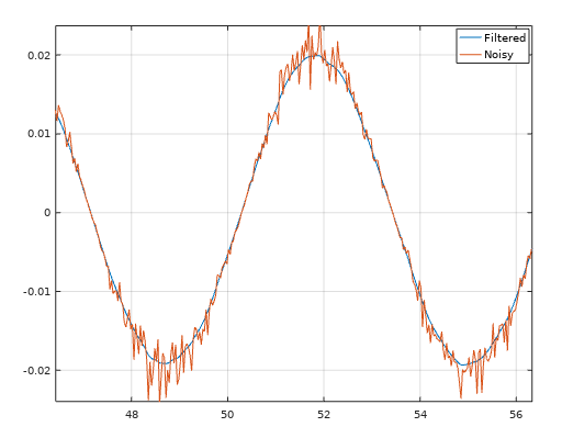
Robust principal component analysis(RPCA) is a great tool if you want to separate noise from data X into a matrix S. RPCA is a better tool than PCA because it using optimization and not only reconstructing the image using SVD, which PCA only does.
[L, S] = rpca(X);clc; clear; close all;
X = imread('..\pictures\bob.png'); % Load Mr Bob
X = rgb2gray(X); % Grayscale 8 bit
X = double(X); % Must be double 40 => 40.0
[L, S] = rpca(X); % Start RPCA. Our goal is to get L matrix
figure(1)
imshow(uint8(X)) % Before RPCA
title('Before RPCA - Bob')
figure(2)
imshow(uint8(L)) % After RPCA
title('After RPCA - Bob')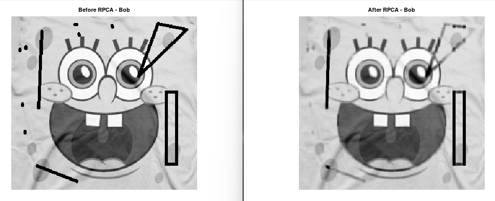
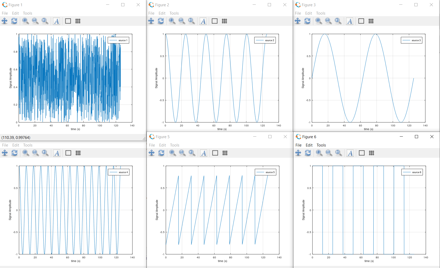
Independent component analysis(ICA) is a tool if you want to separate independent signals from each other. This is not a filter algorithm, but instead of removing noise, it separate the disturbances from the signals. The disturbances are created from other signals. Assume that you have an engine and you are measuring vibration in X, Y and Z-axis. These axis will affect each other and therefore the signals will act like they are mixed. ICA separate the mixed signals into clean and independent signals.
[S] = ica(X);% Clear all plots
clear
close all
clc
% Tick clock
tic
%% Parameters
N = 6; %The number of observed mixtures
M = 1000; %Sample size, i.e.: number of observations
K = 0.1; %Slope of zigzag function
na = 8; %Number of zigzag oscillations within sample
ns = 5; %Number of alternating step function oscillations within sample
finalTime = 40*pi; %Final sample time (s)
initialTime = 0; %Initial sample time (s)
%% Generating Data for ICA
% Create time vector data
timeVector = initialTime:(finalTime-initialTime)/(M-1):finalTime;
% Create random, cos, sin and fast cos signal
source1 = rand(1, M);
source2 = cos(0.25*timeVector);
source3 = sin(0.1*timeVector);
source4 = cos(0.7*timeVector);
% Ziggsack signal
source5 = zeros(1,M);
periodSource5 = (finalTime-initialTime)/na;
for i = 1:M
source5(i) = K*timeVector(i)-floor(timeVector(i)/periodSource5)*K*periodSource5;
end
source5 = source5 - mean(source5);
% PWM signal
source6 = zeros(1,M);
periodSource6 = (finalTime-initialTime)/ns/2;
for i = 1:M
if mod(floor(timeVector(i)/periodSource6),2) == 0
source6(i) = 1;
else
source6(i) = -1;
end
end
source6 = source6 - mean(source6);
% Create our source matrix. This matrix is what want to find
S = [source1;source2;source3;source4;source5;source6];
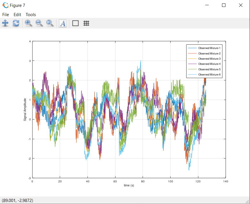
% Create an matrix A that going to mix all signals in S, that we calling X
Amix = rand(N,N);
X = Amix*S;
figure
plot(timeVector,source1)
xlabel('time (s)')
ylabel('Signal Amplitude')
legend('source 1')
figure
plot(timeVector,source2)
xlabel('time (s)')
ylabel('Signal Amplitude')
legend('source 2')
figure
plot(timeVector,source3)
xlabel('time (s)')
ylabel('Signal Amplitude')
legend('source 3')
figure
plot(timeVector,source4)
xlabel('time (s)')
ylabel('Signal Amplitude')
legend('source 4')
figure
plot(timeVector,source5)
xlabel('time (s)')
ylabel('Signal Amplitude')
legend('source 5')
figure
plot(timeVector,source6)
xlabel('time (s)')
ylabel('Signal Amplitude')
legend('source 6')
figure
plot(timeVector,X);
xlabel('time (s)')
ylabel('Signal Amplitude')
legend('Observed Mixture 1', 'Observed Mixture 2', 'Observed Mixture 3', 'Observed Mixture 4', 'Observed Mixture 5', 'Observed Mixture 6')
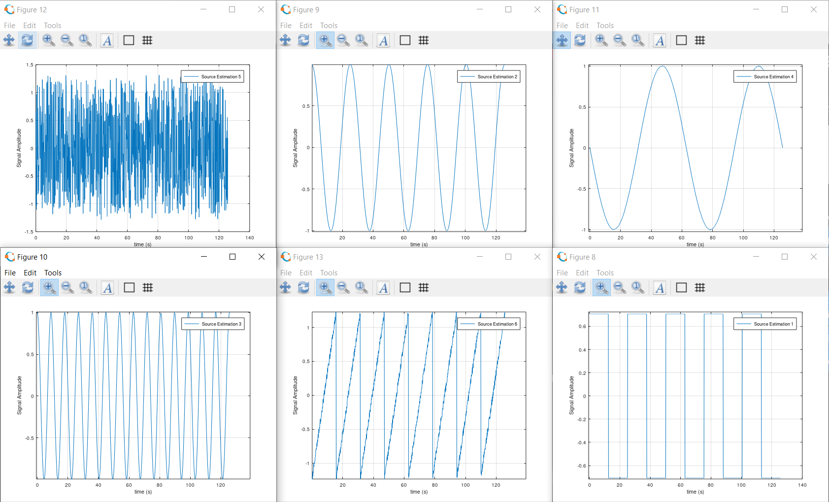
% Use ICA to find S from X
S = ica(X);
figure
plot(timeVector, S(1,:))
xlabel('time (s)')
ylabel('Signal Amplitude')
legend('Source Estimation 1')
figure
plot(timeVector, S(2,:))
xlabel('time (s)')
ylabel('Signal Amplitude')
legend('Source Estimation 2')
figure
plot(timeVector, S(3,:))
xlabel('time (s)')
ylabel('Signal Amplitude')
legend('Source Estimation 3')
figure
plot(timeVector, S(4,:))
xlabel('time (s)')
ylabel('Signal Amplitude')
legend('Source Estimation 4')
figure
plot(timeVector, S(5,:))
xlabel('time (s)')
ylabel('Signal Amplitude')
legend('Source Estimation 5')
figure
plot(timeVector, S(6,:))
xlabel('time (s)')
ylabel('Signal Amplitude')
legend('Source Estimation 6')
% End clock time and check the difference how long it took
tocThese signals are what we want to find
This is how the signals look when we are measuring them
This is how the signals are reconstructed as they were independent
This is Uncented Kalman Filter that using cholesky update method (more stable), instead of cholesky decomposition. This algorithm can estimate parameters to very a complex function if data is available. This method is reqursive and there is a C code version in CControl as well. Use this when you need to estimate parameters to a function if you have data that are generated from that function. It can be for example an object that you have measured data and you know the mathematical formula for that object. Use the measured data with this algorithm and find the parameters for the formula.
[Sw, what] = sr_ukf_parameter_estimation(d, what, Re, x, G, lambda_rls, Sw, alpha, beta, L);% Initial parameters
L = 3; % How many states we have
e = 0.1; % Tuning factor for noise
alpha = 0.1; % Alpha value - A small number like 0.01 -> 1.0
beta = 2.0; % Beta value - Normally 2 for gaussian noise
Re = e*eye(L); % Initial noise covariance matrix - Recommended to use identity matrix
Sw = eye(L); % Initial covariance matrix - Recommended to use identity matrix
what = zeros(L, 1); % Estimated parameter vector
d = zeros(L, 1); % This is our measurement
x = [4.4; 6.2; 1.0]; % State vector
lambda_rls = 1.0; % RLS forgetting parameter between 0.0 and 1.0, but very close to 1.0
% Our transition function - This is the orifice equation Q = a*sqrt(P2 - P1) for hydraulics
G = @(x, w) [w(1)*sqrt(x(2) - x(1));
% We only need to use w(1) so we assume that w(2) and w(3) will become close to 1.0
w(2)*x(2);
w(3)*x(3)];
% Start clock time
tic
% Declare arrays
samples = 100;
WHAT = zeros(samples, L);
E = zeros(samples, L);
% Do SR-UKF for parameter estimation
for i = 1:samples
% Assume that this is our measurement
d(1) = 5 + e*randn(1,1);
% This is just to make sure w(2) and w(3) becomes close to 1.0
d(2) = x(2);
d(3) = x(3);
% SR-UKF
[Sw, what] = sr_ukf_parameter_estimation(d, what, Re, x, G, lambda_rls, Sw, alpha, beta, L);
% Save the estimated parameter
WHAT(i, :) = what';
% Measure the error
E(i, :) = abs(d - G(x, what))';
end
% Stop the clock
toc
% Print the data
[M, N] = size(WHAT);
for k = 1:N
subplot(3,1,k);
plot(1:M, WHAT(:,k), '-', 1:M, E(:, k), '--');
title(sprintf('Parameter estimation for parameter w%i', k));
ylabel(sprintf('w%i', k));
grid on
legend('Estimated parameters', 'Parameter error')
end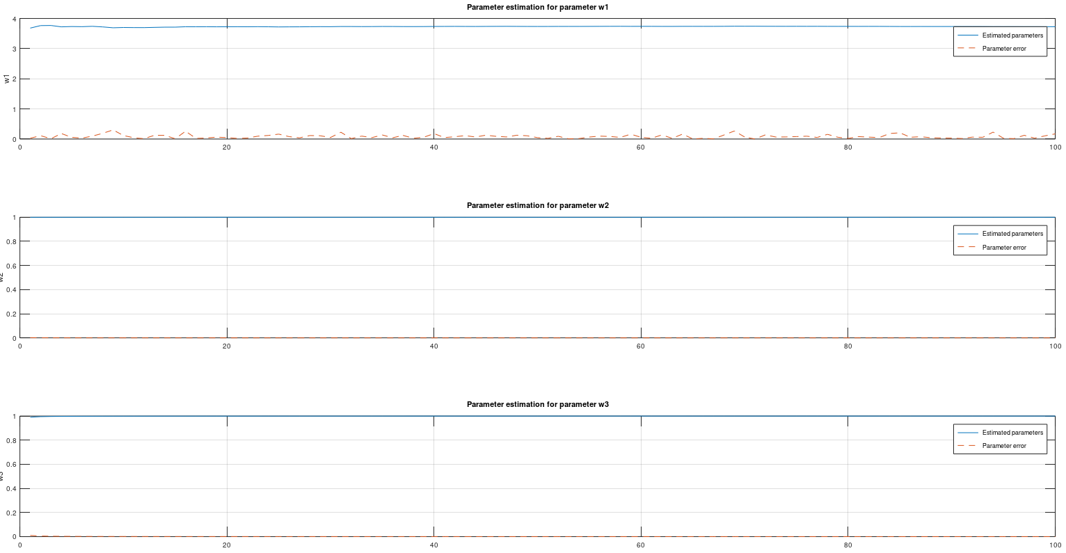
This is Uncented Kalman Filter that using cholesky update method (more stable), instead of cholesky decomposition. This algorithm can estimate states from a very complex model. This method is reqursive and there is a C code version in CControl as well. Use this when you need to estimate state to a model if you have data that are generated from that function. It can be for example an object that you have measured data and you know the mathematical formula for that object. Use the measured data with this algorithm and find the states for the model.
[S, xhat] = sr_ukf_state_estimation(y, xhat, Rn, Rv, u, F, S, alpha, beta, L);% Initial parameters
L = 3; % How many states we have
r = 1.5; % Tuning factor for noise
q = 0.2; % Tuning factor for disturbance
alpha = 0.1; % Alpha value - A small number like 0.01 -> 1.0
beta = 2.0; % Beta value - Normally 2 for gaussian noise
Rv = q*eye(L); % Initial disturbance covariance matrix - Recommended to use identity matrix
Rn = r*eye(L); % Initial noise covariance matrix - Recommended to use identity matrix
S = eye(L); % Initial covariance matrix - Recommended to use identity matrix
xhat = [0; 0; 0]; % Estimated state vector
y = [0; 0; 0]; % This is our measurement
u = [0; 0; 0]; % u is not used in this example due to the transition function not using an input signal
x = [0; 0; 0]; % State vector for the system (unknown in reality)
% Our transition function
F = @(x, u) [x(2);
x(3);
0.05*x(1)*(x(2) - x(3))];
% Start clock time
tic
% Declare arrays
samples = 200;
X = zeros(samples, L);
XHAT = zeros(samples, L);
Y = zeros(samples, L);
phase = [90;180;140];
amplitude = [1.5;2.5;3.5];
% Do SR-UKF for state estimation
for i = 1:samples
% Create measurement
y = x + r*randn(L, 1);
% Save measurement
Y(i, :) = y';
% Save actual state
X(i, :) = x';
% SR-UKF
[S, xhat] = sr_ukf_state_estimation(y, xhat, Rn, Rv, u, F, S, alpha, beta, L);
% Save the estimated parameter
XHAT(i, :) = xhat';
% Update process
x = F(x, u) + q*amplitude.*sin(i-1 + phase);
end
% Stop the clock
toc
% Print the data
[M, N] = size(XHAT);
for k = 1:N
subplot(3,1,k);
plot(1:M, Y(:,k), '-g', 1:M, XHAT(:, k), '-r', 1:M, X(:, k), '-b');
title(sprintf('State estimation for state x%i', k));
ylabel(sprintf('x%i', k));
grid on
legend('y', 'xhat', 'x')
end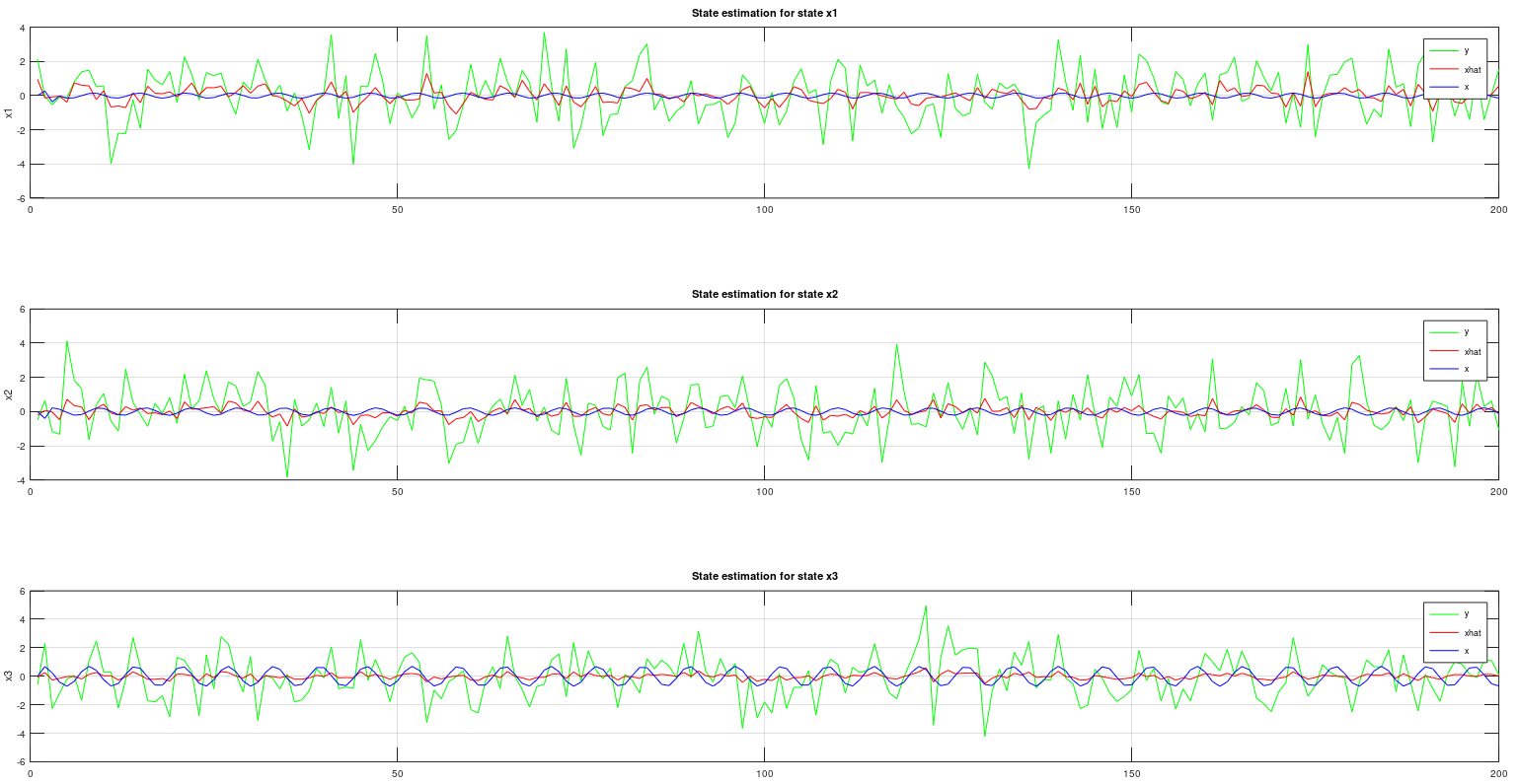
A particle filter is another estimation filter such as Square Root Uncented Kalman Filter (SR-UKF), but SR-UKF assume that the noise is gaussian (normally distributed) and SR-UKF requries a dynamical model. The particle filter does not require the user to specify a dynamical model and the particle filter assume that the noise can be non-gaussian or gaussian, nonlinear in other words.
The particle filter is using Kernel Density Estimation algorithm to create the internal probability model, hence the user only need to specify one parameter with the following example. If you don't have a model that describes the dynamical behaviour, this filter is the right choice for you then.
[xhat, horizon, k, noise] = pf(x, xhatp, k, horizon, noise);% Create inputs
N = 200;
u = linspace(1, 1, N);
u = [5*u 10*u -4*u 3*u 5*u 0*u -5*u 0*u];
% Create time
t = linspace(0, 100, length(u));
% Create second order model
G = tf(1, [1 0.8 3]);
% Simulate outputs
y = lsim(G, u, t);
close
% Add noise
e = 0.1*randn(1, length(u));
y = y + e;
% Do particle filtering - Tuning parameters
p = 4; % Length of the horizon (Change this)
% Particle filter - No tuning
[m, n] = size(y); % Dimension of the output state and length n
yf = zeros(m, n); % Filtered outputs
horizon = zeros(m, p); % Horizon matrix
xhatp = zeros(m, 1); % Past estimated state
k = 1; % Horizon counting (will be counted to p. Do not change this)
noise = rand(m, p); % Random noise, not normal distributed
% Particle filter - Simulation
for i = 1:n
x = y(:, i); % Get the state
[xhat, horizon, k, noise] = pf(x, xhatp, k, horizon, noise);
yf(:, i) = xhat; % Estimated state
xhatp = xhat; % This is the past estimated state
end
% Plot restult
plot(t, y, t, yf, '-r')
grid on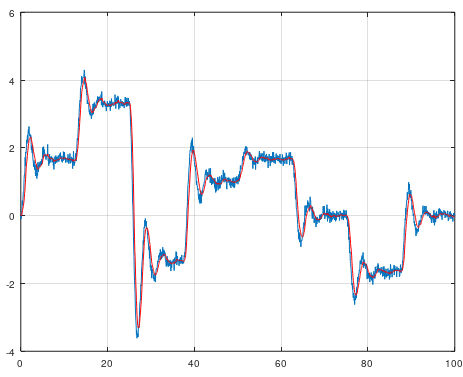
X = dlmread('ParticleFilterDataRaw.csv');
t = X(:, 1)';
y = X(:, 2)';

% Do particle filtering - Tuning parameters
p = 14;                            % Length of the horizon (Change this)

% Particle filter - No tuning
[m, n] = size(y);                  % Dimension of the output state and length n
yf = zeros(m, n);                  % Filtered outputs
horizon = zeros(m, p);             % Horizon matrix
xhatp = zeros(m, 1);               % Past estimated state
k = 1;                             % Horizon counting (will be counted to p. Do not change this)
noise = rand(m, p);                % Random noise, not normal distributed

% Particle filter - Simulation
for i = 1:n
  x = y(:, i);                     % Get the state
  [xhat, horizon, k, noise] = pf(x, xhatp, k, horizon, noise);
  yf(:, i) = xhat;                 % Estimated state
  xhatp = xhat;                    % This is the past estimated state
end

% Plot restult
plot(t, y)
hold on
plot(t, yf, '-r')
grid on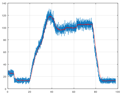
This algorithm can do C code generation for nonlinear models. It's a very simple algorithm because the user set out the support points by using the mouse pointer. When all the supports are set ut, then the algorithm will generate C code for you so you can apply the SVM model in pure C code using CControl library.
All you need to have is two matrices, X and Y. Where the column length is the data and the row length is the amount of classes.
The svm.m file will plot your data and then when you have placed out your support points, then the svm.m will generate C code for you that contains all the support points.
If you have let's say more than two variables, e.g Z matrix or even more. Then you can create multiple models as well by just using diffrent data as arguments for the svm function below. The C code generation is very fast and it's very easy to build a model.
[X_point, Y_point, amount_of_supports_for_class] = svm(X, Y)% How much data should we generate
N = 50;
% How many classes
c = 5;
% Create variance and average for X and Y data
X_variance = [2, 4, 3, 4, 5];
Y_variance = [3, 5, 3, 4, 5];
X_average = [50, 70, 10, 90, 20];
Y_average = [20, 70, 60, 10, 20];
% Create scatter data
X = zeros(c, N);
Y = zeros(c, N);
for i = 1:c
% Create data for X-axis
X(i, 1:N) = X_average(i) + X_variance(i)*randn(1, N);
% Create data for Y-axis
Y(i, 1:N) = Y_average(i) + Y_variance(i)*randn(1, N);
end
% Create SVM model - X_point and Y_point is coordinates for the SVM points.
% amount_of_supports_for_class is how many points there are in each row
[X_point, Y_point, amount_of_supports_for_class] = svm(X, Y);
% Do a quick re-sampling of random data again
for i = 1:c
% Create data for X-axis
X(i, 1:N) = X_average(i) + X_variance(i)*randn(1, N);
% Create data for Y-axis
Y(i, 1:N) = Y_average(i) + Y_variance(i)*randn(1, N);
end
% Check the SVM model
point_counter_list = zeros(1, c);
for i = 1:c
% Get the points
svm_points_X = X_point(i, 1:amount_of_supports_for_class(i));
svm_points_Y = Y_point(i, 1:amount_of_supports_for_class(i));
% Count how many data points this got - Use inpolygon function that return 1 or 0 back
point_counter_list(i) = sum(inpolygon(X(i,:) , Y(i, :), svm_points_X, svm_points_Y));
end
% Plot how many each class got - Maximum N points per each class
figure
bar(point_counter_list);
xlabel('Class index');
ylabel('Points');


To install Mataveid, download the folder "sourcecode" and place it where you want it. Then the following code need to be written in the terminal of your MATLAB® or GNU Octave program.
path('path/to/the/sourcecode/folder/where/all/matave/files/are/mataveid', path)
savepath
Example:
path('/home/hp/Dokument/Reglerteknik/mataveid', path)
savepath
Important! All the .m files need to be inside the folder mataveid if you want the update function to work.
Write this inside the terminal. Then Mataveid is going to download new .m files to mataveid from GitHub
updatemataveid- Installation of Matavecontrol package https://github.com/DanielMartensson/matavecontrol

