This module creates energy level diagrams common to atomic physics as matplotlib graphics. The level structure is defined using networkx graphs.

This package takes networkx directional graphs, which can be used to effectively define a system hamiltonian, and creates an energy diagram representing the system. The nodes of the graph represent the energy levels. The edges of the graph represent the couplings between levels.

Passing a simple graph to the basic level diagram constructor will produce a passable output for simple visualization purposes.

nodes = (0,1,2)
edges = ((0,1),(1,2))
graph = nx.DiGraph()
graph.add_nodes_from(nodes)
graph.add_edges_from(edges)
d = ld.LD(graph)
d.draw()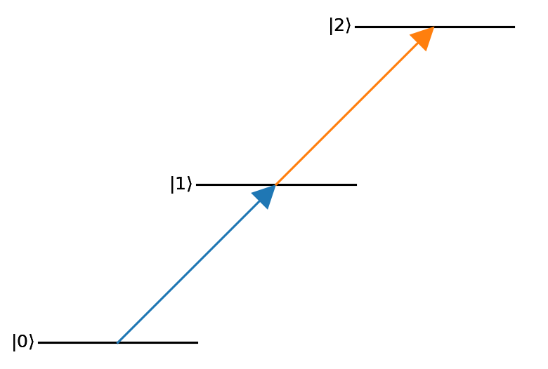

Global settings for the three primitive objects used by leveldiagram can be set by passing keyword argument dictionaries to the LD constructor. To control options for a single level or coupling, save these keyword arguments to the respective node or edge of the supplied graph. Generally, the levels and couplings take standard matplotlib 2D line configuration arguments.

nodes = ((0,{'bottom_text':'ground'}),
         (1,{'right_text':'excited'}),
         (2,{'top_text':'rydberg'}))
edges = ((0,1, {'label':'$\\Omega_p$'}),
         (1,2, {'label':'$\\Omega_c$'}))
graph = nx.DiGraph()
graph.add_nodes_from(nodes)
graph.add_edges_from(edges)
d = ld.LD(graph, coupling_defaults = {'arrowsize':0.15,'lw':3})
d.draw()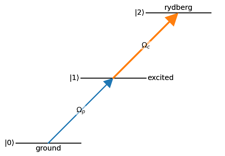

With some basic scripting to create the graph appropriately, much more complicated level diagrams can be made with relative ease.

hf_nodes =  [((f,i), {('top' if f==2 else 'bottom') + '_text':'$m_F='+f'{i:d}'+'$',
                      'energy':f-1,
                      'xpos':i,
                      'width':0.75,
                      'text_kw':{'fontsize':'large'}})
             for f in [1,2]
             for i in range(-f,f+1)]
lin_couples = [((1,i),(2,i),{'label':l,'color':'C0',
                            'label_kw':{'fontsize':'medium','color':'C0'}})
               for i,l in zip(range(-1,2), ['1/2','2/3','1/2'])]
sp_couples = [((1,i),(2,i+1),{'label':l,'color':'C1',
                              'label_offset':'right',
                             'label_kw':{'fontsize':'medium','color':'C1'}})
              for i,l in zip(range(-1,2), ['1/6','1/2','1'])]
sm_couples = [((1,i),(2,i-1),{'label':l, 'color':'C2',
                              'label_offset':'left',
                             'label_kw':{'fontsize':'medium','color':'C2'}})
              for i,l in zip(range(-1,2), ['1','1/2','1/6'])]
hf_edges = lin_couples + sp_couples + sm_couples
hf_graph = nx.DiGraph()
hf_graph.add_nodes_from(hf_nodes)
hf_graph.add_edges_from(hf_edges)
d = ld.LD(hf_graph, default_label = 'none')
d.ax.margins(y=0.2)
d.draw()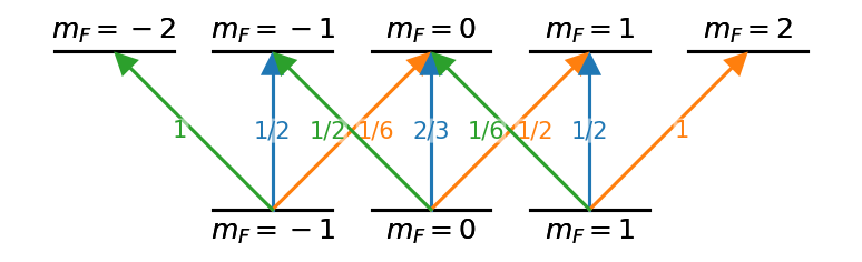

Presently, installation must be done manually using a copy of the repository.

To install in an editable way (which allows edits of the source code), run:

pip install -e .

from within the top level leveldiagram directory (i.e. where the setup.cfg file resides). This command will use pip to install all necessary dependencies.

To install normally, run:

pip install .

from the same directory.

Upgrading an existing installation is simple. Simply run the pip installation commands described above with the update flag.

pip install -U .

This command will also install any new dependencies that are required.

If using an editable install, simply replacing the files in the same directory is sufficient. Though it is recommended to also run the appropriate pip update command as well.

pip install -U -e .

Requires matplotlib, networkx, and numpy.

A PDF copy of the documentation is avaiable in the docs/build/latex/ directory.

Example jupyter notebooks that demonstrate leveldiagrams can be found in the examples subdirectory. Printouts of these notebooks are available in the docs as well.