K-Nearest Neighbors (K-NN) is a non-parametric, instance-based learning algorithm.

Rather than learning a model from the training data, K-NN memorizes the data. To make predictions for new, unseen data points, the algorithm looks up the known, labeled data points (the "nearest neighbors") based on their feature similarity.

1. Select K: Define the number of neighbors, denoted by the hyperparameter $K$.
2. Compute distance: Typically, Euclidean or Manhattan distance is used to identify the nearest data points.
3. Majority vote: For classification, the most common class among the K neighbors is predicted. For regression, the average of the neighbors' values is calculated.

• Euclidean Distance:

$$ \sqrt{\sum_{i=1}^{n}(q_i-p_i)^2} $$

• Manhattan Distance:

$$ \sum_{i=1}^{n}|q_i-p_i| $$

• Simplicity: Easy to understand and implement.
• No Training Period: New data is simply added to the dataset during inference.
• Adaptability: Can dynamically adjust to changes in the data.

• Computationally Intensive: As the algorithm scales, its computational requirements grow.
• Memory Dependent: Storing the entire dataset for predictions can be impractical for large datasets.
• Sensitivity to Outliers: Outlying points can disproportionately affect the predictions.

K-Nearest Neighbors (K-NN) is a straightforward yet effective non-parametric algorithm used for classification and regression. Today, let's focus particularly on its classification abilities.

1. Calculate Distances: Compute the distance between the query instance and all the training samples.

   • Euclidean, Manhattan, Hamming, or Minkowski distances are commonly used.

2. Find k Nearest Neighbors: Select the k nearest neighbors to the query instance based on their distances.

3. Majority Vote: For classification, the most popular class among the selected k neighbors is chosen as the final prediction.

4. Classify the Query Instance: Assign the class to the query by taking the class that's most common among its k nearest neighbors.

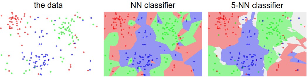
In K-NN, the decision boundary is defined by the areas where there's a transition from one class to another. This boundary is calculated based on the distances of the k-nearest neighbors.

• In two-dimensional space, if $k = 3$, the decision boundary would look like three interconnecting clusters radiating from the classified point.
• As $k$ increases, the decision boundary becomes smoother, potentially leading to lesser overfitting.

The choice of $k$ can substantially impact both the accuracy and the smoothness of the decision boundary. For instance:

• With smaller $k$, there's a higher probability of overfitting since predictions are influenced by just a few neighbors.
• Conversely, with larger $k$, the model might suffer from underfitting as it could become too influenced by the majority class. Therefore, determining the optimal $k$ is crucial for balance.
• Common approaches to $k$ selection include using odd values, such as 1, 3, or 5 for binary classification.

• K-NN can be computationally demanding for high $k$ or in scenarios with a substantial number of training data points (as the distances need to be calculated for each point).

• Without the application of feature scaling, attributes with large scales might unfairly dominate the distance calculation.

• Feature Scaling: Before running K-NN, normalize or scale attributes.
• Outlier Handling: The strategy should be consistent across both the training and test sets.
• Feature Selection: Opting only for the most pertinent attributes could enhance performance and reduce computational cost.

K-Nearest Neighbors (K-NN) is commonly associated with classification tasks, where it excels at non-parametric, instance-based learning. Surprisingly, K-NN can be harnessed just as effectively for regression tasks, where it's known as K-Nearest Neighbors Regressor.

In a regression setting, K-NN calculates the target by averaging or taking the weighted average of the $k$ most similar instances in terms of input features.

The predictor of the K-NN Regressor is obtained through:

$$ \hat{Y}(x) = \frac{1}{k} \sum_{i \in N_k(x)} y_i $$

where $N_k(x)$ is the set of instances $x_i$ from the training dataset that are the nearest to $x$. Here, nearest is defined with respect to some distance metric, most commonly the Euclidean distance.

1. Parameter k Selection: Determine the most effective $k$ for your dataset. Small k values might lead to overfitting, while larger $k$ values could smoothen the predictions.

2. Distance Metric: K-NN can use various distance metrics, such as Euclidean, Manhattan, and Minkowski. Choose the metric that best suits the nature of your data.

3. Feature Scaling: For effective distance calculations, consider normalizing or standardizing the features.

Here is the Python code:

from sklearn.neighbors import KNeighborsRegressor
from sklearn.datasets import load_boston
from sklearn.model_selection import train_test_split
from sklearn.preprocessing import StandardScaler
from sklearn.metrics import mean_squared_error
import numpy as np

# Load Boston dataset
boston = load_boston()
X, y = boston.data, boston.target

# Split the data into training and test sets
X_train, X_test, y_train, y_test = train_test_split(X, y, test_size=0.3, random_state=42)

# Standardize the features
scaler = StandardScaler()
X_train = scaler.fit_transform(X_train)
X_test = scaler.transform(X_test)

# Initialize K-NN Regressor
knn_regressor = KNeighborsRegressor(n_neighbors=5, weights='uniform')

# Fit the model
knn_regressor.fit(X_train, y_train)

# Predict on the test set
y_pred = knn_regressor.predict(X_test)

# Evaluate the model using Mean Squared Error
mse = mean_squared_error(y_test, y_pred)
print(f"Mean Squared Error: {mse}")

# Optionally, you can also perform hyperparameter tuning using techniques like GridSearchCV

In this example, we use the Boston housing dataset and a KNeighborsRegressor from scikit-learn to perform K-NN regression.

'K' in K-NN determines the number of nearest neighbors considered for decision-making. Here is how you choose its value.

1. Manual Choice: For smaller datasets or when computational limitations exist. It's important to perform hyper-parameter tuning to find the optimal K value.

2. Odd vs Even: Prefer odd K-values to avoid tie-breakers in binary classifications.

3. Value Range: Since K typically ranges from 1 to the square root of the total number of data points, one can use heuristics and cross-validation for finer churn.

4. Elbow Method: Visualize K's effect on accuracy through a line plot. Look for a "bend" or "elbow" after which the improvement in accuracy becomes marginal.

5. Cross-Validation: Use techniques like k-fold CV to evaluate the model's performance for different K values. Choose the K that yields the best average performance.

6. Grid Search with Cross-Validation: Automate K selection by performing an exhaustive search over specified K-values using cross-validation.

7. Algorithms for K-Optimization: Some sophisticated techniques like "Isolation Forest" come with built-in methods for selecting the most appropriate K.

K-nearest neighbors (kNN) is a simple and intuitive classification algorithm. It assigns the class most common among the $k$ nearest examples - defined by a chosen distance metric.

• Simplicity: The algorithm is straightforward and easy to implement.
• Interpretability: K-NN directly mimics human decision-making by referencing close neighbors.
• Flexibility: It can adapt over time by including new examples or adjusting $k$.
• Lack of Assumptions: It doesn't require a priori knowledge about the underlying distribution of data or its parameters.
• No Training Period: Most of the time spent with the algorithm is in its testing phase, making it particularly time- and resource-efficient for large or dynamic datasets.

• Computationally Expensive: For each new example, the algorithm needs to compute the distances to all points in the testing dataset. This can be particularly burdensome in large data sets.
• Sensitive to Irrelevant Features: K-NN can be influenced by irrelevant or noisy features, leading to degraded performance.
• Biased Toward Features with Many Categories or High Scales: Attributes with large scales can dominate the distance calculation.
• Need for Optimal $K$: The algorithm's performance can be significantly affected by the choice of $k$.
• Imbalanced Data Can Lead to Biased Predictions: When the classes in the data are imbalanced, the majority class will likely dominate the prediction for new examples.

• Handling Missing Values: K-NN doesn't inherently address missing data, necessitating the use of imputation methods or other strategies.
• Noise Sensitivity: Presence of noisy data can lead to poor classification accuracy.
• Distance Metric Dependence: The selection of the distance metric can significantly impact K-NN's performance. It might be necessary to experiment with different metrics to find the most suitable one for the specific dataset.

While the K-Nearest Neighbors algorithm is simple and intuitive, it might not be the best fit for certain scenarios due to some of its inherent limitations.

• High Computational Cost: Each prediction requires computation of the distances between the new data point and every existing point in the feature space. For large datasets, this can be computationally demanding and time-consuming.

• Need for Feature Scaling: K-NN is sensitive to the scales of the features. Features with larger scales might disproportionately influence the distance-based calculations. Therefore, it's important to standardize or normalize the feature set before leveraging K-NN.

• Imbalanced Data Handling: In the case of an imbalanced dataset (i.e., one where the number of observations in different classes is highly skewed), the predictions can be biased towards the majority class.

• Irrelevant and Redundant Features: K-NN can be impacted by noise and non-informative features, as it treats all features equally. The inclusion of irrelevant and redundant features might lead to biased classifications.

• Curse of Dimensionality: As the number of features or dimensions increases, the data becomes increasingly sparse in the feature space, often making it challenging for K-NN to provide accurate predictions.

Here is the Python code:

from sklearn.neighbors import KNeighborsClassifier
import pandas as pd
import time

# Generate a synthetic dataset
data = pd.DataFrame({
    'feature1': range(1, 1001),
    'feature2': range(1001, 1, -1)
})
data['target'] = data['feature1'] % 2

X, y = data[['feature1', 'feature2']], data['target']
knn_classifier = KNeighborsClassifier(n_neighbors=5)

# Measure time to fit K-NN on large dataset
start_time = time.time()
knn_classifier.fit(X, y)
fit_time = time.time() - start_time
print(f"Time to fit K-NN on 1000 data points: {fit_time:.2f} seconds")

The K-Nearest Neighbors (K-NN) algorithm's effectiveness is heavily influenced by the distance metric chosen. Selecting the most suitable metric is crucial for accurate classification or regression.

1. Euclidean Distance: Standard measure in K-NN and assumes attributes are continuous and have equal importance.

$$ d(x, y) = \sqrt{\sum_{i=1}^{n}(x_i - y_i)^2} $$

2. Manhattan Distance: Also known as "Taxicab" distance or $L_1$ norm. It's useful for high-dimensional data since it calculates the 'city block' or 'L1' distance.

$$ d(x, y) = \sum_{i=1}^{n} |x_i - y_i| $$

3. Minkowski Distance: Generalises both Euclidean and Manhattan metrics. By setting $q=2$, it simplifies to Euclidean, and with $q=1$, it becomes Manhattan.

$$ d(x, y) = \left(\sum_{i=1}^{n} |x_i - y_i|^q\right)^{\frac{1}{q}} $$

4. Chebyshev Distance: Measures the maximum distance along any coordinate axis, providing robust performance in the presence of outliers.

$$ d(x, y) = \max_{i} |x_i - y_i| $$

5. Hamming Distance: Suitable for categorical data, it calculates the proportion of attributes that are not matching.

$$ d(x, y) = \frac{1}{n} \sum_{i=1}^{n} \delta(x_i, y_i) $$

6. Cosine Similarity: Utilized for text and document classification, it measures the cosine of the angle between two vectors.

$$ d(x, y) = 1 - \frac{\sum_{i=1}^{n} x_i \cdot y_i}{\sqrt{\sum_{i=1}^{n} x_i^2} \cdot \sqrt{\sum_{i=1}^{n} y_i^2}} $$

1. Data Type Consideration:

   • For continuous/numeric and mixed data types, Euclidean and Minkowski (with $q=2$) are usually suitable.
   • For high-dimensional data, consider Manhattan or Chebyshev.
   • For categorical data, Hamming yields reliable results.

2. Data Distribution and Outliers:

   • For datasets that are not normalized and contain outliers, consider metrics like Manhattan or Chebyshev.
   • For normalized datasets, Euclidean is a standard choice.

3. Feature Scales:

   • Normalized: Use Euclidean, Manhattan, or Minkowski.
   • Not Normalized: Chebyshev may be preferable.

4. Computational Complexity:

   • For a large dataset with many dimensions, city block distance (Manhattan or Minkowski with q=1) is computationally more efficient.

5. Domain Knowledge:

   • Expertise in the subject area can guide distance metric selection. For instance, in image processing, Manhattan or Minkowski with Chebyshev norms are common.

6. Combine with Cross-Validation:

   • Use techniques such as cross-validation to choose the best metric for your data. This ensures the most suitable metric is chosen while avoiding bias.

7. Python Example: Choosing the Best Metric:

# Import Necessary Libraries
from sklearn.model_selection import cross_val_score
from sklearn.neighbors import KNeighborsClassifier

# Define a k-NN classifier
knn = KNeighborsClassifier(n_neighbors=3)

# Perform Cross-Validation to Evaluate Different Metrics
scores = cross_val_score(knn, X, y, cv=10, scoring='accuracy')

# Print Cross-Validation Scores
print('Accuracy with Euclidean Distance:', scores.mean())

knn = KNeighborsClassifier(n_neighbors=3, p=1)  # Using Manhattan Distance
scores = cross_val_score(knn, X, y, cv=10, scoring='accuracy')
print('Accuracy with Manhattan Distance:', scores.mean())

K-Nearest Neighbors (K-NN) is a non-parametric, instance-based algorithm that uses distance metrics to classify data. While it's not mandatory to perform feature scaling before using the K-NN algorithm, doing so can lead to several practical advantages.

1. Improved Convergence: Algorithms like K-NN that are based on distance metrics might converge faster when features are scaled.

2. Equal Feature Importance: Scaling ensures all features contribute equally to the distance calculation. Without it, features with larger numeric ranges can dominate the distance metric.

3. Better Visualization & Interpretation: Data becomes easier to interpret and visualize when its features are on similar scales. This can be beneficial for understanding the decision boundaries in K-NN.

4. Prevents Bias: Unnormalized features might introduce bias to the distance metric, influencing the classification process.

5. Efficiency: Normalizing or standardizing data can help reduce computation time, especially for high-dimensional datasets.

6. Feature Comparison: Scaled features have similar ranges, making it easier to visualize their relationship through scatter plots.

1. Min-Max Scaling:

$$ x_{\text{norm}} = \frac{x - \text{min}(x)}{\text{max}(x) - \text{min}(x)} $$

All features are bounded within the range of 0 to 1.

3. Z-Score Standardization:

$$ x_{\text{std}} = \frac{x - \bar{x}}{s} $$

• Here, $\bar{x}$ is the mean and $s$ is the standard deviation.
• Features have a mean of 0 and a standard deviation of 1 after scaling.

5. Robust Scaler: Scales features using the interquartile range, making it less sensitive to outliers.

   • Useful when dealing with datasets that have extreme values ("outliers").

6. Max Abs Scaler: Scales features based on their maximum absolute value.

   • It's not impacted by the mean of the data.

7. Unit Vector Scaling: Normalizes features to have unit norm (magnitude).

   • Useful in cases where direction matters more than specific feature values.

8. Power Transformation: Utilizes power functions to make data more Gaussian-like which can enhance the performance of some algorithms.

   • Useful when dealing with data that doesn't follow a Gaussian distribution.

9. Quantile Transformation: It transforms features using information from the quantile function, making it robust to outliers and more normally distributed.

   • Valuable in scenarios where data is not normally distributed or has extreme values.

10. Yeo-Johnson Transformation: A generalized version of the Box-Cox transformation, handling both positive and negative data.

• Useful for features with a mixture of positive/negative values or near-zero values.

11. Data Cleansing: Outliers can be removed, or imputed using various techniques before running K-NN.

12. Discretization: Converting continuous features to discrete ones can sometimes enhance the performance of K-NN, especially with smaller datasets.

Here is a Python code:

from sklearn.preprocessing import MinMaxScaler
from sklearn.neighbors import KNeighborsClassifier
from sklearn.model_selection import train_test_split
from sklearn.metrics import accuracy_score
import pandas as pd

# Load dataset
data = pd.read_csv('your_dataset.csv')
X = data.drop('target_column', axis=1)
y = data['target_column']

# Split data into training and testing sets
X_train, X_test, y_train, y_test = train_test_split(X, y, test_size=0.2, random_state=42)

# Scale features using Min-Max
scaler = MinMaxScaler()
X_train_scaled = scaler.fit_transform(X_train)
X_test_scaled = scaler.transform(X_test)

# Train K-NN classifier
knn = KNeighborsClassifier(n_neighbors=5)
knn.fit(X_train_scaled, y_train)

# Predictions
y_pred = knn.predict(X_test_scaled)

# Accuracy
accuracy = accuracy_score(y_test, y_pred)
print(f'Accuracy: {accuracy}')

When it comes to handling multi-class problems, K-Nearest Neighbors (K-NN) typically adopts one of the following two strategies:

For multi-class classification:

• OneHotEncoding: The output classes are often represented using one-hot encoded vectors, where each class is a unique sequence of binary values (e.g., [1,0,0], [0,1,0], and [0,0,1] for a 3-class problem). The predicted class is the one that results in the smallest distance.
• Hamming Distance: A distance metric designed for one-hot encoded vectors. It calculates the number of positions in two equal-length binary numbers that are different.

For scenarios where K-NN is not the most effective or efficient choice, consider the following techniques:

• Ensemble Methods: Techniques like Bagging (Bootstrap Aggregating) which involves combining the decisions from multiple models to increase overall accuracy. Meta-estimators like the multi-class version of K-NN from the scikit-learn Python library integrates these techniques.

• Dimensionality Reduction: Utilize methods like Principal Component Analysis (PCA) to reduce the model's input attributes.

While K-Nearest Neighbors $K-NN$ is primarily for classification and regression, it can assist in a rudimentary form of feature selection through the curse of dimensionality.

The curse of dimensionality refers to challenges in high-dimensional spaces, such as excessive computational and sample size requirements. These difficulties can hinder K-NN's performance and that of other machine learning algorithms.

With an increased number of dimensions, the distance between neighboring data points becomes less meaningful, making it harder for the algorithm to distinguish patterns.

• Distance Measures: K-NN relies on distance metrics like Euclidean or Manhattan distance to determine nearest neighbors. In high-dimensional spaces, these metrics can become less effective, a phenomenon known as non-metricity. To mitigate this, feature scaling or normalization can be applied.

• Feature Selection: By choosing a subset of the most relevant features, the apparent "closeness" of instances can be more reliable.

  There exist several methods for feature selection and feature engineering, aimed at improving model performance by reducing noise and computational overhead. Using a smaller number of informative features can help combat dimensionality-related challenges.

Despite these strategies, K-NN isn't designed primarily for feature selection. You can still use techniques like Univariate Feature Selection, Recursive Feature Elimination, or Principal Component Analysis to reduce dimensionality.

These techniques can be employed in conjunction with K-NN to potentially enhance its predictive accuracy.

For dimensionality reduction with techniques like PCA, you might encounter a trade-off where the interpretability of feature importance is lost. In such a scenario, it might be more effective to use a dedicated feature selection mechanism, especially when interpretability is crucial.

Ultimately, while K-NN can provide some inherent feature selection benefits, utilizing it alongside dedicated feature selection methods can enhance model performance.

Weighted K-Nearest Neighbors (K-NN) is a variation of the K-NN algorithm that computes predictions through a weighted combination of the k-nearest neighbor classes.

This approach outperforms the standard K-NN approach in scenarios where individual neighbors may have varying levels of importance or relevance in the decision-making process. Weighted K-NN enables different neighbors to carry uneven weights, based on their relevance to the prediction.

• Relevance Assessment: Assigns higher significance to neighbors whose attributes more closely match those of the data point being classified.

• Local Embedding: Emphasizes neighbors that are in closer proximity to the data point, contributing to a more locally refined decision boundary.

• Inverse Distance: The weight of each neighbor is determined by the inverse of its distance to the data point: $\weight( x_i ) = \frac{1}{d( \mathbf{x}_i, \mathbf{x} )}$

• Distance Square Root: Weights are computed using the square root of the inverse of the distances: $\weight( x_i ) = \frac{1}{\sqrt{d( \mathbf{x}_i, \mathbf{x} )}}$

• Gaussian Radial Basis Function (RBF): Employs the Gaussian RBF curve, which assigns weight based on the distance between the data point and its neighbor: $\weight( x_i ) = e^{-\frac{1}{2\sigma^2} d( \mathbf{x}_i, \mathbf{x} )}$

• User-Defined Functions: In some implementations, custom functions can be used to calculate weights, offering flexibility in the weighting strategy.

Here is the Python code:

import numpy as np
from collections import Counter

def weighted_knn(X_train, y_train, x, k, weight_func):
    distances = [np.linalg.norm(x - x_train) for x_train in X_train]
    idx = np.argsort(distances)[:k]
    k_nearest_labels = [y_train[i] for i in idx]
    weights = [weight_func(x, X_train[i]) for i in idx]
    weighted_votes = Counter({label: 0 for label in np.unique(y_train)})
    
    for label, weight in zip(k_nearest_labels, weights):
        weighted_votes[label] += weight
        
    return weighted_votes.most_common(1)[0][0]

The curse of dimensionality refers to various challenges that arise when dealing with high-dimensional feature spaces. It has significant implications for K-nearest neighbors (K-NN) algorithms.

• Increased Sparsity: With many dimensions, data points tend to spread out, making it harder to discern meaningful patterns.

• Diminishing Discriminatory Power: As dimensions increase, the relative difference between pairwise distances diminishes.

• Computational Burden: Nearest neighbor search becomes more resource-intensive in high-dimensional spaces.

1. Feature Selection and Extraction:

   • Focus on a subset of features relevant to the task.
   • Employ techniques like Principal Component Analysis (PCA).

2. Feature Engineering:

   • Derive new features or combine existing ones in a manner that reduces dimensionality.

3. Dimensionality Reduction Techniques:

   • Algorithms such as t-distributed Stochastic Neighbor Embedding (t-SNE) and Uniform Manifold Approximation and Projection (UMAP) can project high-dimensional data into lower dimensions for visualization and K-NN.

4. Rethinking the Problem:

   • Explore if the high dimensionality is truly necessary for the task at hand.

5. Use Distance Metrics Optimized for High Dimensions:

   • Techniques like Locality-Sensitive Hashing (LSH) can improve efficiency in high-dimensional spaces.

6. Increasing the Number of Training Data Points:

   • While not decreasing dimensionality, it may help in understanding the underlying pattern.

K-Nearest Neighbors (K-NN) is a lazy, non-parametric algorithm suitable for both classification and regression tasks. However, its performance can be affected by imbalanced datasets.

1. Performance Degradation: K-NN might exhibit low precision, recall, or accuracy. This is because the algorithm favors the majority class during classification.

2. Inefficient Decision Boundaries: Nearest Neighbors are more likely to belong to the majority class. Consequently, the decision boundaries might not accurately delineate the minority class, leading to smaller support.

3. Distance Bias: Minority class samples, which are crucial for identifying true neighbors, might be treated as outliers. This happens because Euclidean distance measures assume all features are equally significant. When feature scales are different, the calculated distances are dominated by those in higher-impact dimensions.

4. Parity Conflict: In the presence of mixed features (e.g., numerical and categorical), it might be unclear which distance measure to employ, leading to unequal feature considerations.

1. Resampling: Balance the dataset by either oversampling the minority class or undersampling the majority class.

2. Feature Engineering: Transform or assemble features to alleviate bias towards high-scaled ones.

3. Data Augmentation: Introduce synthetic data, particularly for minority classes, to better reflect reality.

4. Algorithm Adaptation: Use modified versions of K-NN, such as WK-NN, which weighs the contributions of neighbors based on their distances.

5. Advanced Techniques: Leverage ensemble methods (e.g., EasyEnsemble, Balance Cascade) or consider cost-sensitive learning, where K-NN is trained to minimize a custom cost function that accounts for class imbalance.

Locality-Sensitive Hashing (LSH) is a data reduction technique that can speed up K-Nearest Neighbors (K-NN) search in high-dimensional spaces by avoiding the computation of distances between all data points.

• K-NN Search Problem: For a given query point $q$, find the $k$ closest points from a dataset $D$, according to a specified distance metric $d$.
• LSH Approach: Preprocess $D$ with a hash function to map points to "buckets" probabilistically, such that if two points are close, they are likely to be in the same or nearby buckets.

1. MinHash for Approximate Nearest Neighbors: Suitable for large text or DNA datasets, it approximates similarities.
2. Random Projections: Efficient for high-dimensional datasets, it uses a set of random vectors to create hash bins. If a point is in front of the vector, the hash function assigns it to one bin; otherwise, it's assigned to a different bin.

Here is the Python code:

from datasketch import MinHash, MinHashLSH

# Sample texts
text_data = [
    "LSH is an LSH-based technique!",
    "Locality-Sensitive Hashing is super cool.",
    "Nearest Neighbor is a related search problem."
]

# Initialize LSH
lsh = MinHashLSH(threshold=0.5, num_perm=128)

# Create MinHash for each text & add to LSH index
for i, text in enumerate(text_data):
    minhash = MinHash(num_perm=128)
    for word in text.split():
        minhash.update(word.encode('utf8'))
    lsh.insert(str(i), minhash)

# Query for closest text to a new input
query_text = "Similarity search in high dimensions"
new_minhash = MinHash(num_perm=128)
for word in query_text.split():
    new_minhash.update(word.encode('utf8'))
result_set = lsh.query(new_minhash, 1)
print("Approximate Nearest Neighbor:", text_data[int(result_set.pop())])

K-Nearest Neighbors (K-NN) and Radius Nearest Neighbors (R-NN) are both instances of the $k$-NN algorithm, designed to handle different tasks and input data. While K-NN identifies the closest $k$ neighbors based on user-defined distance, R-NN frees itself of a static $k$ and instead focuses on neighbors within a specified radius.

• Operational Efficiency: R-NN can be more efficient in computations because it doesn't have to evaluate as many distances as K-NN within the neighborhood (depending on the dimensionality of the data and other factors).
• Varying Neighborhood Density: R-NN allows for more intuitive handling of datasets with differing local densities, whereas K-NN is limited to a fixed count of neighbors.

• Dynamic Neighborhood: R-NN updates the count of neighbors as per the dataset, while K-NN does not adjust the static $k$ count.
• Parameter Setting: K-NN offers a single hyperparameter ($k$) to tune, while R-NN presents the choice of two: the radius and the number of neighbors within.

Here is the Python code:

from sklearn.neighbors import RadiusNeighborsClassifier

# Create and fit a R-NN model
rnn = RadiusNeighborsClassifier(radius=0.5, outlier_label=1)
rnn.fit(X_train, y_train)

# Predict on new data
rnn.predict(X_test)

• When to Choose K-NN:

  • Balanced Data: Suitable when the class distributions in the dataset are fairly uniform.
  • Fixed Neighborhood: Appropriate for scenarios where a consistent count of nearest neighbors is desired.

• When to Choose R-NN:

  • Varied Class Densities: Effective in datasets where different regions have unequal densities of target classes.
  • Dynamic Neighborhood: Best when the number of nearest neighbors can vary within the dataset.

• K-NN with Adaptive Neighborhood: Some implementations, like Variants of k-NN (VkNN), aim to combine the best of both worlds. They adjust the neighborhood size dynamically, using either a radius-based approach or an $f$-nearest neighbors mechanism, making it efficient for high-dimensional datasets.

  • Exact Modified K-NN (EMkNN): A version of $k$-NN that determines the number of nearest neighbors adaptively for each target, reducing the computation time.