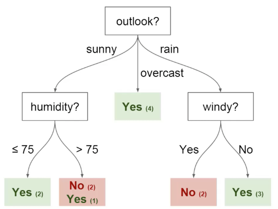
A Decision Tree is a fundamental classification and regression algorithm in machine learning. It partitions the feature space into distinctive subspaces using a tree structure defined by binary, categorical-splits.

• Root Node: Represents the entire dataset. It indicates the starting point for building the tree.
• Internal Nodes: Generated to guide data to different branches. Each node applies a condition to separate the data.
• Leaves/Decision Nodes: Terminal nodes where the final decision is made.

• Partitioning: Data is actively stratified based on feature conditions present in each node.
• Recursive Process: Splitting happens iteratively, beginning from the root and advancing through the tree.

• Gini Impurity: Measures how often the selected class would be mislabeled.
• Information Gain: Calculates the reduction in entropy after data is split. It selects the feature that provides the most gain.
• Reduction in Variance: Used in regression trees, it determines the variance reduction as a consequence of implementing a feature split.

• Interpretable: Easily comprehended, requiring no preprocessing like feature scaling.
• Handles Non-Linearity: Suitable for data that doesn't adhere to linear characteristics.
• Efficient with Multicollinearity and Irrelevant Features: Their performance does not significantly deteriorate when presented with redundant or unimportant predictors.

• Overfitting Sensitivity: Prone to creating overly complex trees. Regularization techniques, like limiting the maximal depth, can alleviate this issue.
• High Variance: Decision trees are often influenced by the specific training data. Ensembling methods such as Random Forests can mitigate this.
• Unbalanced Datasets: Trees are biased toward the majority class, which is problematic for imbalanced categories.

Here is the Python code:

from sklearn.tree import DecisionTreeClassifier
from sklearn.model_selection import train_test_split
from sklearn.metrics import accuracy_score

# Load dataset (e.g., Iris)
# X = features, y = target
X_train, X_test, y_train, y_test = train_test_split(X, y, test_size=0.2, random_state=42)

# Define the model
model = DecisionTreeClassifier()

# Fit the model
model.fit(X_train, y_train)

# Make predictions
y_pred = model.predict(X_test)

# Evaluate accuracy
accuracy = accuracy_score(y_test, y_pred)
print(f"Accuracy: {accuracy:.2f}")

The decision tree uses a top-down, recursive strategy. The tree begins with a single node that evaluates the entire dataset. Each parent node then "decides" the best way to split the data. The process repeats until the nodes or subsets are pure — secured under a single class or meet halting conditions.

• Entropy: A measure of impurity in a set of labels. Decision trees aim to reduce entropy by split.
• Information Gain: The entropy reduction achieved by a data split. The attribute yielding the highest gain is typically chosen.
• Gini Index: Another measure of impurity, similar to entropy, which decision trees can use instead.
• Leaf Node: A node at the end of the tree that doesn't split the data any further. All samples reaching a leaf belong to the same target class.

Here is the Python code:

from math import log2

# Calculate the entropy of a dataset
def calculate_entropy(data):
    total_count = len(data)
    label_counts = {}
    for row in data:
        label = row[-1]
        if label not in label_counts:
            label_counts[label] = 0
        label_counts[label] += 1
    entropy = 0
    for count in label_counts.values():
        probability = count / total_count
        entropy -= probability * log2(probability)
    return entropy

# Calculate information gain for a feature in a dataset
def calculate_information_gain(data, feature_index):
    entropy_before_split = calculate_entropy(data)
    unique_values = set(row[feature_index] for row in data)
    entropy_after_split = 0
    for value in unique_values:
        subset = [row for row in data if row[feature_index] == value]
        subset_entropy = calculate_entropy(subset)
        weight = len(subset) / len(data)
        entropy_after_split += weight * subset_entropy
    return entropy_before_split - entropy_after_split

# Example usage
data = [['Sunny', 85, 85, False, 'No'],
        ['Sunny', 80, 90, True, 'No'],
        ['Overcast', 83, 86, False, 'Yes'],
        ['Rainy', 70, 96, False, 'Yes'],
        ['Rainy', 68, 80, False, 'Yes']]
ig = calculate_information_gain(data, 0)  # Calculate IG for the first feature (Outlook)
print(ig)

Decision Trees serve various machine learning tasks. Here, we'll differentiate between their use for classification and regression.

Classifcation Decision Trees are primarily employed for tasks with discrete target variables. They're especially useful for rapidly separating data into distinctive, non-overlapping categories.

A company uses a Decision Tree to identify customer segments as "high-potential" and "low-interest."

• Gini Index: Focuses on optimizing splits by reducing class impurity.
• Information Gain: Measures the extent of reduction in entropy after the dataset is split.

Here is the Python code:

from sklearn.tree import DecisionTreeClassifier
tree_clf = DecisionTreeClassifier()
tree_clf.fit(X, y)

Unlike their classification counterparts, Regression Decision Trees are best suited for continuous target variables and function by defining prediction points based on a unique set of features.

A real-estate firm might use a Decision Tree to estimate a property's sale price.

• Variance Reduction: Quantifies the drop in variance achieved following a dataset split.
• Mean-Squared Error (MSE): Measures the average squared difference between the predicted values and the actual values.

Here is the Python code:

from sklearn.tree import DecisionTreeRegressor
tree_reg = DecisionTreeRegressor()
tree_reg.fit(X, y)

Several algorithms are designed for constructing Decision Trees.

Let's look at four popular ones:

• Splitting Criterion: Uses information gain or gain ratio as a base, which can lead to biases towards features with more unique categories.
• Handling Missing Data: Not natively supported.
• Numerical Data Handling: Suitable for attribute-values on a discrete domain (requiring categorical data).

• Splitting Criterion: Employs Gini impurity or information gain.
• Handling Missing Data: It is possible, and typically the algorithm decides where to classify observations where data is missing.
• Numerical Data Handling: Binary recursive splitting based on whether a logical test, e.g., 'feature < 6', is met.

• Splitting Criterion: Utilizes the chi-square statistic to detect interactions between variables and resulting multi-way splits for categorical predictors.
• Handling Missing Data: Able to operate with missing fields.
• Numerical Data Handling: Primarily for categorical data, but ordinal variables (both discrete and continuous) can also be utilized.

• Splitting Criterion: Employs the sum of least squares (SLS) as the primary method to minimize error for a continuous target variable.
• Handling Missing Data: Offers options like surrogate split points to handle missing data.
• Numerical Data Handling: Designed particularly for smooth, piecewise polynomial functions but can be extended and modified to account for categorical predictors.

Decision Trees are dynamic, versatile algorithms with several distinct advantages:

• User-Friendly Nature: They are intuitively understood and require little data preparation, making them a go-to choice for exploratory modeling.

• Support for Both Numerical and Categorical Input: This feature simplifies both data preparation and interpretation.

• Efficiency in Time and Space: Decision Trees are among the fastest algorithms, which is an advantage on big data.

• Interpretability: Their transparent nature allows both analysts and regulatory officers to understand the decision-making process.

• Robustness Against Outliers and Missing Values: Decision Trees can handle these issues without external treatment.

• Feature Importance: By calculating attribute metrics such as Gini impurity or information gain, Decision Trees highlight the most salient features, aiding in interpretability and feature selection.

• Tree Pruning for Enhanced Generalization: Techniques like Reduced Error Pruning or Cost-Complexity Pruning refine Decision Trees, mitigating overfitting and fostering better predictive accuracy.

• Model Transparency: Decision Trees are especially effective for generating white-box models, making their decisions clear and easy to follow, ensuring explainability and auditability for sensitive applications.

• Combining Models with Ensemble Methods: Decision trees can be aggregated into advanced models such as Random Forests, Gradient Boosted Trees, XGBoost, AdaBoost for even better performance.

• Risk Assessment and Classification: Decision Trees can be used to stratify risk in scenarios like healthcare, financial evaluations, or predictive maintenance.

• Visual Representation: Graphical summaries of the decision logic make them a powerful tool for data analysis and presentation.

While Decision Trees have several advantages, they also come with a set of limitations and challenges.

1. Overfitting: Unrestrained, decision trees can perfectly fit training data, leading to poor generalization. Techniques like pruning or using ensemble methods mitigate this.

2. Bias Toward Dominant Classes: In datasets with imbalanced class distribution, these trees tend to favor majority classes, which can lead to classification errors for the minority classes.

3. Sensitive to Noise: Even small amounts of noise can create a high level of complexity, leading to spurious predictions. Preprocessing techniques, such as data cleaning, can help here.

4. Non-robust Splitting: The choice of the "best" attribute to split on can vary significantly with minor changes in the dataset. Multiple trees through ensemble methods can help in this regard.

5. Not Suitable for Non-binary Outcomes: While extensions exist, traditional decision trees handle classification problems with only binary outcomes.

6. Feature Correlation Handling: Traditional decision trees can miss identifying correlated features that could be strong predictors in combination. Ensuring acyclic graphs can alleviate this.

7. Data Partitioning Challenges: Decision trees can struggle with segments containing data points with similar characteristics.

   For example, in a two-dimensional feature space, a decision tree might create a partition that is suboptimal when considering both feature axes simultaneously.

8. Subjectivity to Splits and Metrics: The process of determining which attribute to split on (feature selection) and the best split point (threshold selection) might lead to subjectivity, especially when using Gini impurity or information gain metrics.

To mitigate these challenges, various techniques and advanced versions of decision trees are available. Some of these include:

1. Ensemble Methods: Techniques like Random Forests or Boosting build multiple trees and aggregate their predictions, providing improved robustness, generalization, and accuracy.

2. Feature Scaling and Selection: Standardizing features to a common scale and identifying the most relevant ones can enhance tree performance.

3. Pruning: Limiting tree depth post-construction or removing nodes that do not improve overall tree performance helps to avoid overfitting.

4. Dealing with Imbalanced Data: Techniques like SMOTE (Synthetic Minority Over-sampling Technique) or using specialized ensemble approaches like Balanced Random Forests, are designed to handle imbalanced datasets.

5. Cross-Validation: Assessing tree performance on unseen data by splitting the dataset into multiple folds aids in understanding generalization errors.

6. Cost-Complexity Pruning: A variant of traditional pruning that considers the cost (usually misclassification costs) associated with subtrees, leading to better models.

7. Use of Other Tree Models: Enhanced decision tree models like C4.5 (which also handles non-binary outcomes) or CART have been developed to build on the shortcomings of earlier models.

While building a Decision Tree, the algorithm selects the feature that best splits the dataset at each node. This selection is based on minimizing the impurity or maximizing the information gain.

Impurity quantifies the degree of "mixing" of classes within a dataset or a subset. In classification, impurity helps measure the homogeneity of a set of labels:

• A dataset is pure if it contains only one class or label.
• A dataset is impure if it contains an even mixture of classes.

Common impurity metrics in Decision Trees include:

1. Gini Impurity: Measures the probability of misclassifying an instance by randomly assigning a label according to the class distribution. It is in the range of $[0, 0.5]$.

$$ G = 1 - \sum_{i=1}^{n} p_i^2 $$

2. Entropy: Reflects the amount of disorder in a system. It is mathematically similar to Gini impurity and also ranges from 0 (pure) to 1 (impure).

$$ H = - \sum_{i=1}^{n} p_i \log(p_i) $$

3. Misclassification Error: Represents the proportion of majority-class data points, predicting the majority class for all instances. This metric is in the range $[0, 0.5]$.

$$ E = 1 - \max(p_1, p_2, \ldots, p_n) $$

Here is the Python code:

import numpy as np

# Gini impurity
def gini(p):
    return 1 - np.sum(p**2)

# Entropy
def entropy(p):
    return -np.sum(p * np.log(p))

# Misclassification error
def misclassification_error(p):
    return 1 - max(p)

# Class probabilities
p = np.array([0.4, 0.6])

# Calculate impurity measures
gini_impurity = gini(p)
entropy_impurity = entropy(p)
misclassification_error_impurity = misclassification_error(p)

print("Gini Impurity:", gini_impurity)
print("Entropy:", entropy_impurity)
print("Misclassification Error:", misclassification_error_impurity)

In the context of Decision Trees, entropy and information gain are key concepts used to measure the effectiveness of splitting a dataset.

Kullback-Leibler divergence, $H(p)$, provides a principled approach to measuring information or surprise in datasets.

In the context of decision trees, we often compute the entropy, $H(S)$, for a given dataset $S$ characterized by two classes (e.g., "yes"/"no", "spam"/"not spam"):

$$ H(S) = -p \log_2(p) - (1-p) \log_2(1-p) $$

where $p$ is the probability of one class in the dataset.

Information gain (IG) represents the reduction in entropy or uncertainty after a dataset is split by the attribute $A$:

$$ IG(S, A) = H(S) - \sum_{v \in Values(A)} \frac{|S_v|}{|S|} H(S_v) $$

where $S_v$ is the subset of $S$ for which attribute $A$ has value $v$.

Lower entropy values and higher information gain values translate to more effective, rule-based dataset partitions in decision trees.

Gini impurity is a metric used in Decision Trees to evaluate the "purity" of a split.

The Gini impurity is employed at each split point in a decision tree to determine which feature and split value to use. The goal is to find the split that minimizes the impurity by maximizing the information gain.

$$ \text{Gini}(p) = 1 - \sum_{i=1}^J p(i)^2 $$

where:

• $J$ is the number of target classes.
• $p(i)$ represents the probability of a randomly selected sample being correctly classified as class $i$.

1. Squaring Probabilities: Square the probabilities of each class.
2. Summation: Sum the squared probabilities.
3. Subtraction: Subtract the result from 1.

• Computationally Efficient: Gini impurity does not require the expensive computation of logarithms, making it faster to calculate than other impurity measures such as entropy.
• Interpretability: The resulting Gini score has a direct, intuitive meaning and is easier to interpret in the context of decision trees.

Suppose a node has 25 samples, 10 of class A and 15 of class B:

$$ $$ \text{Probability}(\text{Class A}) &= \frac{10}{25} = 0.4 \\ \text{Probability}(\text{Class B}) &= \frac{15}{25} = 0.6 $$ $$

Using these probabilities:

$$ $$ \text{Gini Impurity} &= 1 - \left(\left(0.4\right)^2 + \left(0.6\right)^2\right) \\ &= 1 - \left(0.16 + 0.36\right) \\ &= 1 - 0.52 \\ &= 0.48 $$ $$

So the Gini impurity of this node is 0.48.

Decision Trees are versatile classifiers that can effectively handle both categorical and numerical data. Techniques for processing these data types include Gini impurity, Information Gain, and the use of binary splits.

1. Gini Impurity:

   • For categorical variables: This measures misclassification when more than two categories are present. Categories are directly used for calculating the impurity.
   • For numerical variables: It handles binary classification by converting the numerical value into a binary outcome (e.g., "above" or "below" a certain threshold) and then calculates impurity as if it were a binary categorical variable.

2. Information Gain:

   • For categorical variables: Evaluates reduction in entropy or information uncertainty after particular categorizations.
   • For numerical variables: Uses a binary split to convert the numerical variable into a two-way categorical variable. It's commonly applied using the Gini index in binary mode, whereby the point yielding the highest information gain is chosen as the splitting point.

• Categorical Data: Each distinct category represents a unique branch under a parent node. A data point enters the branch corresponding to its category.

• Numerical Data: Uses binary splits to convert continuous numerical values into ordered categories. The benefit of binary splitting is that only two new branches are created at each node, which simplifies decision-making and visualization.

Here is the Python code:

from sklearn.tree import DecisionTreeClassifier
import pandas as pd

# Sample dataset incorporating both numerical and categorical features
data = {
    'Salary': [50000, 80000, 30000, 70000, 62000],  # Numerical
    'Education': ['Bachelors', 'Masters', 'High School', 'PhD', 'Masters'],  # Categorical
    'Employed': ['Yes', 'Yes', 'No', 'No', 'Yes']  # Categorical
}

# Converting to DataFrame for easier handling
df = pd.DataFrame(data)

# Creating the Decision Tree classifier
tree_clf = DecisionTreeClassifier()

# Fitting the classifier to the dataset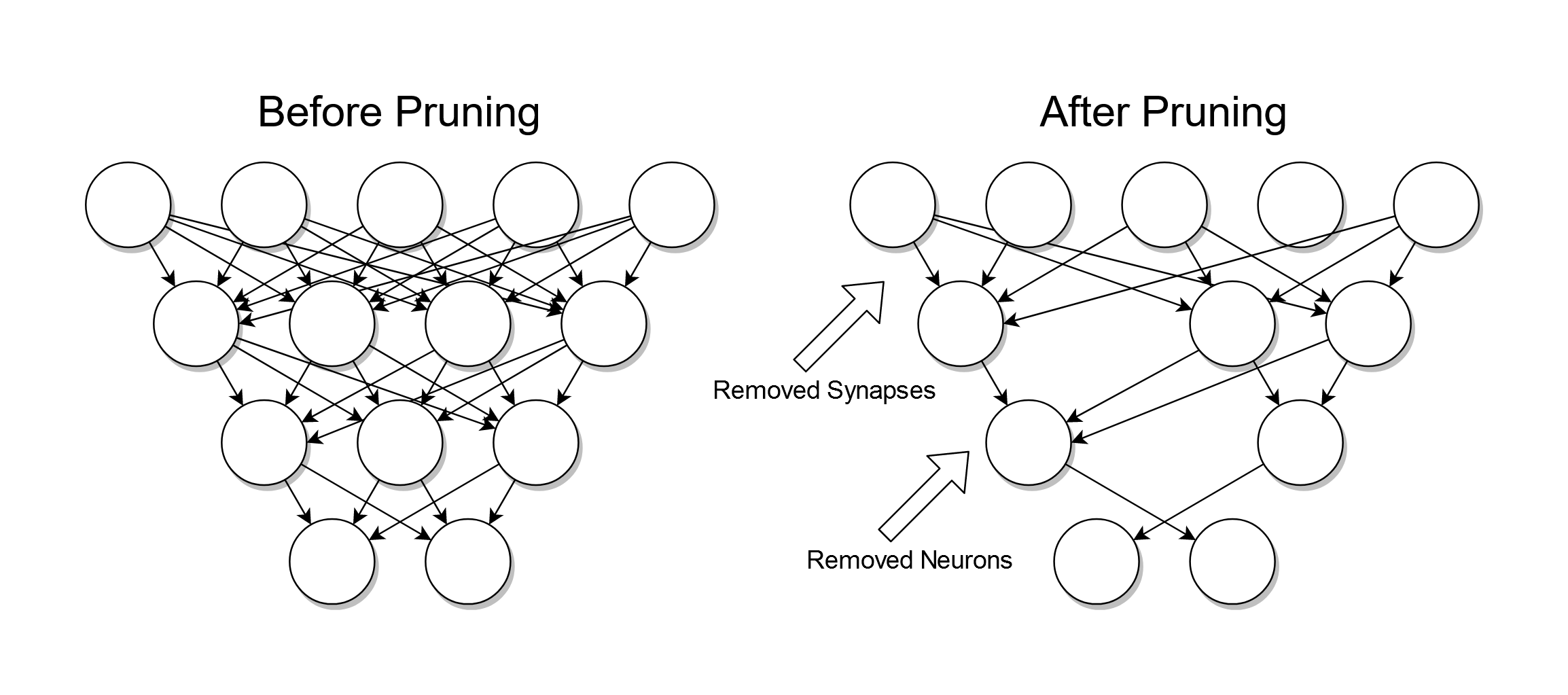
tree_clf.fit(df, ['Yes', 'No', 'No', 'Yes', 'Yes'])

Tree pruning involves the removal of non-essential branches to streamline and optimize decision trees. This optimization is crucial in reducing overfitting and resource demands, while improving model generalization.

Uses stopping criteria to prevent further expansion of branches. This could be based on metrics such as Gini impurity, information gain, or a minimum number of data points.

Entails expanding the tree until each leaf's data points fall under a certain threshold and then working backward to eliminate unnecessary subtrees.

This technique calculates the error on both non-leaf nodes and their corresponding leaf nodes. If pruning a node decreases the overall error, it's pruned.

Also known as "weakest link pruning," this method involves assigning a 'cost' to each node based on error rates and complexity. Pruning occurs if the total cost is reduced.

Instead of completely removing a subtree, grafting sees whether a simplified version of the child would have a better fit within its parent through statistical tests.

• Reduction of Overfitting: By removing noise and unwanted decisions, pruned trees are less likely to overfit to the training data.
• Resource Efficiency: Pruned trees are smaller in size, thereby requiring fewer computational resources for operations like classification and tree traversal.
• Improved Interpretability: With fewer decision nodes, the simplified tree is easier to interpret, making it easier for users and stakeholders to understand and trust model predictions.
• Enhanced Generative Power: Pruned trees focus more on predictive and discriminative power, contributing towards better generalization to unseen data.

Decision Trees employ strategies to prevent overfitting by ensuring a simpler, more generalized structure. This prevents the tree from becoming too complex and tailored to the training data, while maintaining its predictive accuracy.

Decision trees can be pruned, during or after construction, to remove unnecessary or redundant segments that are likely to result in overfitting.

Pruning can be conducted using:

• Cost-Complexity Pruning: This method involves assigning a price to each leaf node and internal node. It starts with a large tree, and as the cost decreases, the trees are pruned, allowing only those nodes to be removed that result in lower costs.
• Minimum Cost-Complexity Pruning: This strategy prunes the tree by limiting the growth of nodes that are likely to increase overall tree complexity.

To further combat overfitting, decision trees can be optimized using more advanced methodologies such as feature selection, ensemble methods like Random Forest or Gradient Boosting, and by experimenting with improved evaluation metrics.

Here is the Python code:

from sklearn.datasets import load_iris
from sklearn.tree import DecisionTreeClassifier
from sklearn.model_selection import train_test_split
import matplotlib.pyplot as plt

# Load the iris dataset and split it into training and test sets
iris = load_iris()
X, y = iris.data, iris.target
X_train, X_test, y_train, y_test = train_test_split(X, y, test_size=0.3, random_state=42)

# Create and fit a decision tree classifier using the Gini index for impurity measure
dt = DecisionTreeClassifier(criterion='gini', random_state=42)
dt.fit(X_train, y_train)

# Visualize the tree before pruning
plt.figure(figsize=(20,20))
plot_tree(dt, filled=True, feature_names=iris.feature_names, class_names=iris.target_names)
plt.show()

# Use cost-complexity pruning to prune the tree
path = dt.cost_complexity_pruning_path(X_train, y_train)
ccp_alphas, impurities = path.ccp_alphas, path.impurities
dts = []
for ccp_alpha in ccp_alphas:
    dt = DecisionTreeClassifier(random_state=42, ccp_alpha=ccp_alpha)
    dt.fit(X_train, y_train)
    dts.append(dt)

# Visualize the first tree after pruning
plt.figure(figsize=(20,20))
plot_tree(dts[0], filled=True, feature_names=iris.feature_names, class_names=iris.target_names)
plt.show()

The depth of a Decision Tree directly affects its predictive performance and computational efficiency.

• Model Plurality: The tree represents uncertainty better with more branches and fewer samples in each, resulting in a clearer decision boundary.

• Increased Accuracy: More thorough data segregation leads to more accurate predictions. However, this improvement tapers off beyond a certain depth.

• Computational Overheads: Both training and inference times escalate with enhanced depth, turning the model sluggish and resource-intensive.

Decision Trees may exhibit overfitting if they grow to unmanageable depths, implying an excessive adaptation to the training dataset, at the cost of generalizability. Algorithms like ID3 and CART offer some in-built mechanisms for counteracting this tendency.

Tree Pruning is a post-growth technique that maximizes efficiency and generalizability of Decision Trees. It accomplishes this by removing unnecessary leaf nodes.

Cross-Validation, a pivotal model validation approach, helps Decision Tree fitting by determining the most suitable tree depth. This method tests and gauges model performance across various tree depths and estimates the one with the best fitting.

Decision Trees have a built-in mechanism for handling missing data. This feature makes them attractive for practical use with real-world datasets, which often contain missing values.

In a Decision Tree algorithm, nodes are split based on the feature that provides the most information gain. However, they can also deal with missing data in two primary ways: they can make a decision based on the majority class, or they can distribute the sample to child nodes based on available feature values or some other global criteria.

• Gini Impurity and Information Gain Measurement: By using these metrics, nodes can be split in a way that minimizes impurity and maximizes information gain, even when dealing with missing data.

• Majority Class Voting: If a certain feature has missing values for some of the samples in a node, the algorithm can use the majority class of those samples to make a decision about that feature.

• Distribution Across Child Nodes: The algorithm may send samples with missing values in a particular feature to both child nodes based on, say, a probabilistic approach, where the probability of falling into each node is proportional to the impurity of that node.

Here is the Python code:

from sklearn.tree import DecisionTreeClassifier
from sklearn.datasets import load_iris
import pandas as pd

# Load the dataset
data = load_iris()
X = pd.DataFrame(data.data, columns=data.feature_names)
y = data.target

# Create a Decision Tree
dtree = DecisionTreeClassifier()

# Train the model
dtree.fit(X, y)

# Make predictions
# Note: the model can handle missing data during the prediction phase as well.
# For pre-processing the data, you may use imputer from sklearn.preprocessing
# Here, we intentionally set some values in the input to NaN to simulate missing data.

X_with_missing_values = X.copy()
X_with_missing_values.iloc[::2, 1] = float('nan')

print("Input data with missing values:")
print(X_with_missing_values.head(10))

predictions = dtree.predict(X_with_missing_values)
print("Predictions:")
print(predictions)

Yes, Decision Trees can accommodate multi-output tasks, and are specifically referred to as Multi-Output Trees.

This technique is particularly useful when dealing with problems that necessitate the simultaneous prediction of multiple target variables.

Multi-Output Trees enable the grouping of several dependent variables, such as:

• Non-Correlated Responses: When predictions across targets aren't significantly correlated.
• Categorical and Continuous Features: For datasets with mixed types of data.

Here is the Python code:

from sklearn.datasets import make_regression
from sklearn.model_selection import train_test_split
from sklearn.tree import DecisionTreeRegressor
import numpy as np

# Create multi-output regression data
X, y = make_regression(n_samples=100, n_features=5, n_outputs=3, random_state=42)

# Split data into training and testing sets
X_train, X_test, y_train, y_test = train_test_split(X, y, random_state=42)

# Fit a multi-output Decision Tree Regressor
regr_ = DecisionTreeRegressor()
regr_.fit(X_train, y_train)

# Predict on test set
y_pred = regr_.predict(X_test)

# Check R-squared score
r2_score = regr_.score(X_test, y_test)
print("R-squared score: {:.2f}".format(r2_score))