The package FRK is now at v2.1.0 and available on CRAN! To install, please type

install.packages("FRK")

To install the most recent (development) version, first please install INLA from https://www.r-inla.org/download, then please load devtools and type

install_github("andrewzm/FRK", dependencies = TRUE, build_vignettes = TRUE)

A document containing a description, details on the underlying maths and computations for the EM algorithm (only applicable for Gaussian data), as well as several examples, is available as a vignette titled "FRK_intro". Another vignette, "FRK_non-Gaussian", summarises the maths in a non-Gaussian setting, and contains a couple of examples using non-Gaussian data and the newly available plotting methods. To load these vignettes please type

library("FRK")
vignette("FRK_intro")
vignette("FRK_non-Gaussian")

A paper with more details is available here, and a draft paper detailing the approach in a non-Gaussian setting is available here. If you use FRK in your work, please cite it using the information provided by citation("FRK").

Package: FRK

Type: Package

Title: Fixed Rank Kriging

Version: 2.0.1

Date: 2021-05-26

Author: Andrew Zammit-Mangion, Matthew Sainsbury-Dale

Maintainer: Andrew Zammit-Mangion [email protected]

Description: Fixed Rank Kriging is a tool for spatial/spatio-temporal modelling and prediction with large datasets. The approach decomposes the field, and hence the covariance function, using a fixed set of r basis functions, where r is typically much smaller than the number of data points (or polygons) m. This low-rank basis-function representation facilitates the modelling of 'big' spatial/spatio-temporal data. The method naturally allows for non-stationary, anisotropic covariance functions. Discretisation of the spatial domain into so-called basic areal units (BAUs) facilitates the use of observations with varying support (i.e., both point-referenced and areal supports, potentially simultaneously), and prediction over arbitrary user-specified regions. The package FRK caters for Gaussian and non-Gaussian data, employing a spatial generalised linear mixed model (GLMM) framework to cater for Poisson, binomial, negative-binomial, gamma, and inverse-Gaussian distributed data. FRK also supports inference over various manifolds, including the 2D plane and 3D sphere, and it provides helper functions to model, fit, predict, and plot with relative ease. Zammit-Mangion and Cressie (2021) describe FRK in a Gaussian setting, and detail it's use of basis functions and BAUs.

• Cressie, N., & Johannesson, G. (2008). Fixed rank kriging for very large spatial data sets. Journal of the Royal Statistical Society: Series B, 70, 209–226.
• Zammit-Mangion A, Cressie N (2021). “FRK: an R package for spatial and spatio-temporal prediction with large datasets.” Journal of Statistical Software, In press.

License: GPL (>= 2)

library("FRK")
library("sp")
library("ggplot2")
library("ggpubr")

## Setup
m <- 1000                                                  # Sample size
RNGversion("3.6.0"); set.seed(1)                           # Fix seed
zdf <- data.frame(x = runif(m), y= runif(m))               # Generate random locs
zdf$z <- sin(8 * zdf$x) + cos(8 * zdf$y) + 0.5 * rnorm(m)  # Simulate data
coordinates(zdf) = ~x+y                                    # Turn into sp object

## Run FRK
S <- FRK(f = z ~ 1,                         # Formula to FRK
         list(zdf),                         # All datasets are supplied in list
         n_EM = 10)                         # Max number of EM iterations
pred <- predict(S)                          # Prediction stage

## Plotting
plot_list <- plot(S, pred)
ggarrange(plotlist = plot_list, nrow = 1, legend = "top")

Here we analyse simulated Poisson data. We signify a Poisson data model with a mean response that is modelled using the square-root link function by setting response = "poisson" and link = "sqrt" in FRK(). Other non-Gaussian response distributions available in FRK are the binomial, negative-binomial, gamma, and inverse-Gaussian distributions.

## Simulate Poisson data using the previous example's data to construct a mean 
zdf$z <- rpois(m, lambda = zdf$z^2)

## Run FRK
S <- FRK(f = z ~ 1, list(zdf),                          
         response = "poisson",         # Poisson data model
         link = "sqrt")                # square-root link function
pred <- predict(S)                            

## Plotting
plot_list <- plot(S, pred$newdata)
ggarrange(plot_list$z, plot_list$p_mu, plot_list$interval90_mu, 
          nrow = 1, legend = "top")
             

We now analyse spatio-temporal data, using the NOAA dataset.

## Setup
data("NOAA_df_1990")
Tmax <- subset(NOAA_df_1990, month %in% 7 & year == 1993)
Tmax <- within(Tmax, {time = as.Date(paste(year,month,day,sep="-"))})
STObj <- stConstruct(x = Tmax, space = c("lon","lat"), time = "time", interval = TRUE)

## BAUs: spatial BAUs are 1x1 pixels, temporal BAUs are 1 day intervals
BAUs <- auto_BAUs(manifold = STplane(), 
                       cellsize = c(1, 1, 1),    
                       data=STObj, tunit = "days")
BAUs$fs <- 1 # scalar fine-scale variance matrix, implicit in previous examples

## Basis functions
G <- auto_basis(manifold = STplane(), data = STObj, nres = 2, tunit = "days")

## Run FRK
STObj$std <- 2 # fix the measurement error variance
S <- FRK(f = z ~ 1 + lat, data = list(STObj), 
         basis = G, BAUs = BAUs, est_error = FALSE, method = "TMB")
pred <- predict(S, percentiles = NULL)

## Plotting: include only some times via the argument subset_time
plot_list <- plot(S, pred$newdata, subset_time = c(1, 7, 13, 19, 25, 31)) 
ggarrange(plotlist = plot_list, nrow = 1, legend = "top") 

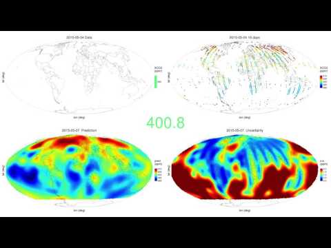
The package FRK is currently being used to generate spatio-temporal animations of fields observed by satellite data. Here we show a daily prediction of CO2 using data from the NASA OCO-2 between September 2014 and June 2016.

Thanks to Michael Bertolacci for designing the FRK hex logo!