The best R package for running NetLogo simulation
From the previous blog, you might have noticed the rationale of using high performance computing (HPC), and how fast it is to obtain results compared to our local machines. Having installed all the software requirements on the HPC, today's post is to simulate a NetLogo model of my Ph.D work in R using an nlrx package(https://ropensci.github.io/nlrx/).
nlrx has promoted its uniqueness for adopting .XML to excecute files that contain various conditions (i.e. runtime, variables, constants, stop conditions), as well as reporting results framed as a BehaviorSpace format. As a passionate NetLogo user, I have to give both thumbs up to this package (psst..! and removed other NetLogo packages). Here are the reasons.
nlrx introduces codes that are catchy and intuitive. Here is a brief example of my model on Windows. If you want a model embedded in the NetLogo library, please refer to the nlrx website.
Prior to loading your model, you have to follow 3 steps: 1) install package(we will skip that), 2) setup, 3) assign variables and conditions, and 4) Plots and animation.
After the installation, your job is to assign your paths correctly. You will need to assign paths for Java, NetLogo, model files, and simulation output. In my case, I wrote the absolute paths to avoid error since softwares and the model are saved in different directories. I use NetLogo 6.0.4, but anyone who is using a different version can modify the version name.
# Java setup
Sys.setenv(JAVA_HOME='C:/Program Files/Java/jdk1.8.0_202/jre') # Windows
Sys.setenv(JAVA_HOME= "/Library/Java/JavaVirtualMachines/jdk1.8.0_212.jdk/Contents/Home/jre/") # MacOSX
Sys.setenv(JAVA_HOME= "/usr/lib/jvm/java-11-openjdk-amd64") # ubuntu
Sys.setenv(JAVA_HOME='/usr/local/software/spack/spack-0.11.2/opt/spack/linux-rhel7-x86_64/gcc-5.4.0/jdk-8u141-b15-p4aaoptkqukgdix6dh5ey236kllhluvr/jre') #Ubuntu cluster


#install.packages("nlrx")
library(nlrx)
# Assign Path
netlogopath <- file.path("C:/Program Files/NetLogo 6.0.4")
outpath <- file.path("d:/out")
# Create nl variable
nl <- nl(nlversion = "6.0.4",
         nlpath = netlogopath,
         modelpath = file.path("D:/github/jasss/Gangnam_v6.nlogo"),
jvmmem = 1024)Now the experiment is where the central function has to be properly defined. That is, you will need to decide everything that you've set in your model. Here is a list of questions:
expname: What is the name of your experiment?outpath: What is the name of your output path?repetition: How many repetitions you want to run?tickmetrics: Would you like to activate ticks?idsetup: Setup button of your modelidgo: Go button of your modelruntime: How many ticks to run (in your model)? e.g. 8764evalticks: Specifying ticks to report. I wanted to capture agent's personal info in every 100 ticks.constants: What is your fixed parameters. pollution standard, pollution scenario (make sure you put your strings inside the backslash!)variables: list of changable parameters. I used factoral variablesmetrics.turtles: turtles and their attributesmetrics.patches: patches and their attributesstopcond: When you need stop conditions
Once every parameter are written, you can test if the model is valid to run the simulation. The package uses eval_variables_constants(nl), and the command will return wheter it is valid or not. Then, we give a simple design simdesign_simple() where constants are used. Finally, with the run_nl_all() command, the model will execute and assign it in the R global environment as result. A kind note is that the result variable is a nested data frame which is heavy and needs to be unnested.
nl@experiment <- experiment(expname = "seoul",
                            outpath = outpath,
                            repetition = 1,
                            tickmetrics = "true",
                            idsetup = "setup",
                            idgo = "go",
                            runtime = 8764,
                            evalticks=seq(1,8764, by = 100),
                            constants = list("PM10-parameters" = 100,
                                             "Scenario" = "\"BAU\"", # Business-as-usual Pollution scenario that repeats the oscilation of existing data
                                             "scenario-percent" = "\"inc-sce\"",
                                             'AC' = 100),
                            #variables = list('AC' = list(values=c(100,150,200))),
                            metrics.turtles =  list("turtles" = c("xcor", "ycor", "color", "heading", "who",
                                                 "homename", "destinationName", "age", "health")),
                            metrics.patches = c("pxcor", "pycor", "pcolor"))


# Evaluate if variables and constants are valid:
eval_variables_constants(nl)
nl@simdesign <- simdesign_simple(nl = nl, nseeds = 1)
# Run Simulation
init <- Sys.time()
results <- run_nl_all(nl = nl)
Sys.time() - init
In short, I think that the developers have made the commands concise and understandable to users in any level.
Another part, which might seem less important but is actually not, is the file size. On the previous section, I mentioned that it runs on a XML file and the results is given as a nested data frame. Surprisingly, the .RData of my simulation result is only 24MB although I have to acknowledge that it took more than 10GB of your memory during the process. Thus if any of you are running NetLogo on Windows, then the first thing you need to do is to increase your virtual memory memory.limit(size = 99999). If you are using Linux or Mac, I really wish you have a good storage of RAM with a generously allocated swap space to run expensive models.
Compared to nlrx, RNetLogo has a while command that records your global variables as a data frame. It used to be good, but they had problems to assigning string variables , which made the user convert it in NetLogo and comback to R for implementation. Moreover, RNetLogo's .RData was more than a 100MB for a single iteration which is okay for a local machine, but might be quite excessive if you are working with peers on a version control.
# Attach results to nl object:
setsim(nl, "simoutput") <- results

# Report spatial data:
results_unnest <- unnest_simoutput(nl)(filter individuals whose health are under 100)
## Load packages
library(tidyverse)
library(gganimate)
library(cartography)
library(rcartocolor)
library(ggthemes)


turtles <- results_unnest %>%
               select(`[step]`, Scenario, xcor, ycor, age, agent, health) %>%
               filter(agent == "turtles",
                      Scenario == "BAU",
                      ycor < 324 & xcor < 294 & xcor > 0,
                      health <= 100) %>%
               filter(`[step]` %in% seq(5000,8764))

patches <- results_unnest %>% select(`[step]`, Scenario, pxcor, pycor, pcolor) %>%
            filter(Scenario == "BAU", pycor < 324 , `[step]` %in% seq(5181,8701,10))


# Create facet plot:
ggplot() +
  facet_wrap(~`[step]`, ncol= 10) +
  coord_equal() +
  geom_tile(data=patches, aes(x=pxcor, y=pycor, fill=pcolor), alpha = .2) +
  geom_point(data=turtles, aes(x = xcor, y = ycor, color = age), size=1, show.legend = FALSE) +
  scale_fill_gradient(low = "white", high = "grey20") +
  scale_color_manual(breaks=c("young", "active", "old"),
                     values = c("young" = "#56B4E9", "active" = "#E69F00", "old" = "#999999")) +
  guides(fill=guide_legend(title="PM10")) +
  ggtitle("Unhealthly Population after a long-term exposure") +
  theme_minimal() +
  theme(axis.line=element_blank(),
        axis.text.x=element_blank(),
        axis.text.y=element_blank(),
        axis.ticks=element_blank(),
        #axis.title.x=element_blank(),
        #axis.title.y=element_blank(),legend.position="none",
        #panel.background=element_blank(),panel.border=element_blank(),panel.grid.major=element_blank(),
        #panel.grid.minor=element_blank(),plot.background=element_blank()
        )
turtles %>%
  group_by(`[step]`, age) %>%
  tally() %>%
  print(n = length(turtles$age)) %>%
  reshape2::dcast(`[step]` ~ age) -> turtle.stat

turtle.stat$total <- rowSums(turtle.stat[,c(2:4)], na.rm = T)| [step] | active | old | young | total |
|---|---|---|---|---|
| 5201 | NA | 3 | 1 | 4 |
| 5301 | NA | 21 | 9 | 30 |
| 5401 | NA | 49 | 26 | 75 |
| 5501 | NA | 49 | 27 | 76 |
| 5601 | NA | 47 | 24 | 71 |
| 5701 | NA | 48 | 25 | 73 |
| 5801 | NA | 45 | 25 | 70 |
| 5901 | NA | 52 | 27 | 79 |
| 6001 | NA | 49 | 27 | 76 |
| 6101 | NA | 51 | 27 | 78 |
| 6201 | NA | 49 | 27 | 76 |
| 6301 | NA | 39 | 25 | 64 |
| 6401 | NA | 37 | 25 | 62 |
| 6501 | NA | 50 | 27 | 77 |
| 6601 | NA | 51 | 27 | 78 |
| 6701 | NA | 51 | 27 | 78 |
| 6801 | 3 | 46 | 23 | 72 |
| 6901 | 10 | 43 | 21 | 74 |
| 7001 | 14 | 43 | 20 | 77 |
| 7101 | 7 | 42 | 19 | 68 |
| 7201 | 11 | 34 | 18 | 63 |
| 7301 | 46 | 39 | 20 | 105 |
| 7401 | 61 | 34 | 19 | 114 |
| 7501 | 65 | 38 | 28 | 131 |
| 7601 | 65 | 43 | 57 | 165 |
| 7701 | 65 | 45 | 69 | 179 |
| 7801 | 63 | 41 | 37 | 141 |
| 7901 | 56 | 36 | 25 | 117 |
| 8001 | 53 | 41 | 35 | 129 |
| 8101 | 61 | 42 | 51 | 154 |
| 8201 | 65 | 51 | 97 | 213 |
| 8301 | 65 | 51 | 97 | 213 |
| 8401 | 61 | 50 | 91 | 202 |
| 8501 | 55 | 47 | 78 | 180 |
| 8601 | 45 | 38 | 63 | 146 |
| 8701 | 47 | 39 | 64 | 150 |
#Density map
turtles_density <- results_unnest %>%
  select(`[step]`, Scenario, xcor, ycor, age, agent, health) %>%
  filter(agent == "turtles", Scenario == "BAU", ycor < 324 & xcor < 294 & xcor > 0) %>%
  filter(`[step]` %in% seq(1,8764))


turtles_density$health[turtles_density$health <= 0] <- 0

turtles_density %>%
  filter() %>%
  ggplot(aes(health, fill = age)) +
  geom_density(aes(y = ..count..), alpha = 0.25) +
  theme_bw(`[step]` == 8701) +
  theme(legend.title = element_text(size=20, face="bold"),
        legend.text = element_text(size=15),
        legend.position = c(0.2, 0.8),
        axis.text=element_text(size=20),
        axis.title=element_text(size=15,face="bold")
  )

library(gganimate)
p1 <- ggplot() +
  geom_tile(data=patches, aes(x=pxcor, y=pycor, fill=factor(pcolor))) +
  geom_point(data=turtles, aes(x = pxcor, y = pycor, group=who, color = breed), size=2) +
  scale_fill_gradient(low = "white", high = "grey20") +
  scale_color_manual(breaks=c("young", "active", "old"),
                     values = c("young" = "#56B4E9", "active" = "#E69F00", "old" = "#999999")) +
  guides(fill=guide_legend(title="PM10")) +
  transition_time(`[step]`) +
  coord_equal() +
  labs(title = 'Step: {frame_time}') +
  theme_void()


# Animate the plot and use 1 frame for each step of the model simulations
gganimate::animate(p1, nframes = length(unique(patches$`[step]`)), width=400, height=400, fps=4)
anim_save("seoul.gif")Codes are not yet reproducible (apologies)!
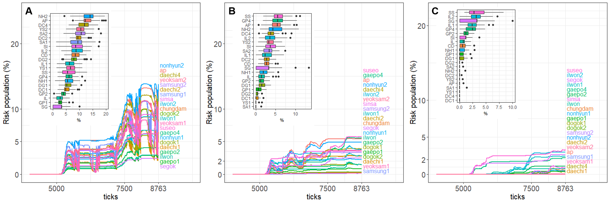
b100 <- plotbl100 + annotation_custom(grob = ggplotGrob(plotbb100), xmin = 4000, xmax = 7500, ymin = 20, ymax = 60)
b150 <- plotbl150 + annotation_custom(grob = ggplotGrob(plotbb150), xmin = 4000, xmax = 7500, ymin = 20, ymax = 60)
b200 <- plotbl200 + annotation_custom(grob = ggplotGrob(plotbb200), xmin = 4000, xmax = 7500, ymin = 20, ymax = 60)

i100 <- plotil100 + annotation_custom(grob = ggplotGrob(plotib100), xmin = 4000, xmax = 7500, ymin = 20, ymax = 60)
i150 <- plotil150 + annotation_custom(grob = ggplotGrob(plotib150), xmin = 4000, xmax = 7500, ymin = 20, ymax = 60)
i200 <- plotil200 + annotation_custom(grob = ggplotGrob(plotib200), xmin = 4000, xmax = 7500, ymin = 20, ymax = 60)

d100 <- plotdl100 + annotation_custom(grob = ggplotGrob(plotdb100), xmin = 4000, xmax = 7500, ymin = 20, ymax = 60)
d150 <- plotdl150 + annotation_custom(grob = ggplotGrob(plotdb150), xmin = 4000, xmax = 7500, ymin = 20, ymax = 60)
d200 <- plotdl200 + annotation_custom(grob = ggplotGrob(plotdb200), xmin = 4000, xmax = 7500, ymin = 20, ymax = 60)


plot_grid(b100, b150, b200, labels = c("A", "B", "C"), ncol = 3, align = "h")
plot_grid(i100, i150, i200, labels = c("D", "E", "F"), ncol = 3, align = "h")
plot_grid(d100, d150, d200, labels = c("G", "H", "I"), ncol = 3, align = "h")