Giter Club home page Giter Club logo

sindy's Introduction

SINDy

Discovering the governing equations of nonlinear systems purely from data using the SINDy method (https://www.pnas.org/content/113/15/3932).

Lorenz system simulation with feedforward strongly nonlinear inputs. This simulation data was used for identification. https://user-images.githubusercontent.com/55796835/127328774-a1342b36-4729-4225-8e3e-fd447fc66a5e.mp4

Lorenz system simulation with feedback inputs. Used for demonstration of identification of a controlled system. Note that the state gravitates more strongly to the right attractor, where it's being pushed by the control law. https://user-images.githubusercontent.com/55796835/127328914-39fbc4ed-b294-48a5-9ac7-729e497d5644.mp4

Simulation of the reference Lorenz model and the model identified from its measurement data. https://user-images.githubusercontent.com/55796835/127679128-65357765-4e09-4b51-9d53-e436224f4084.mp4

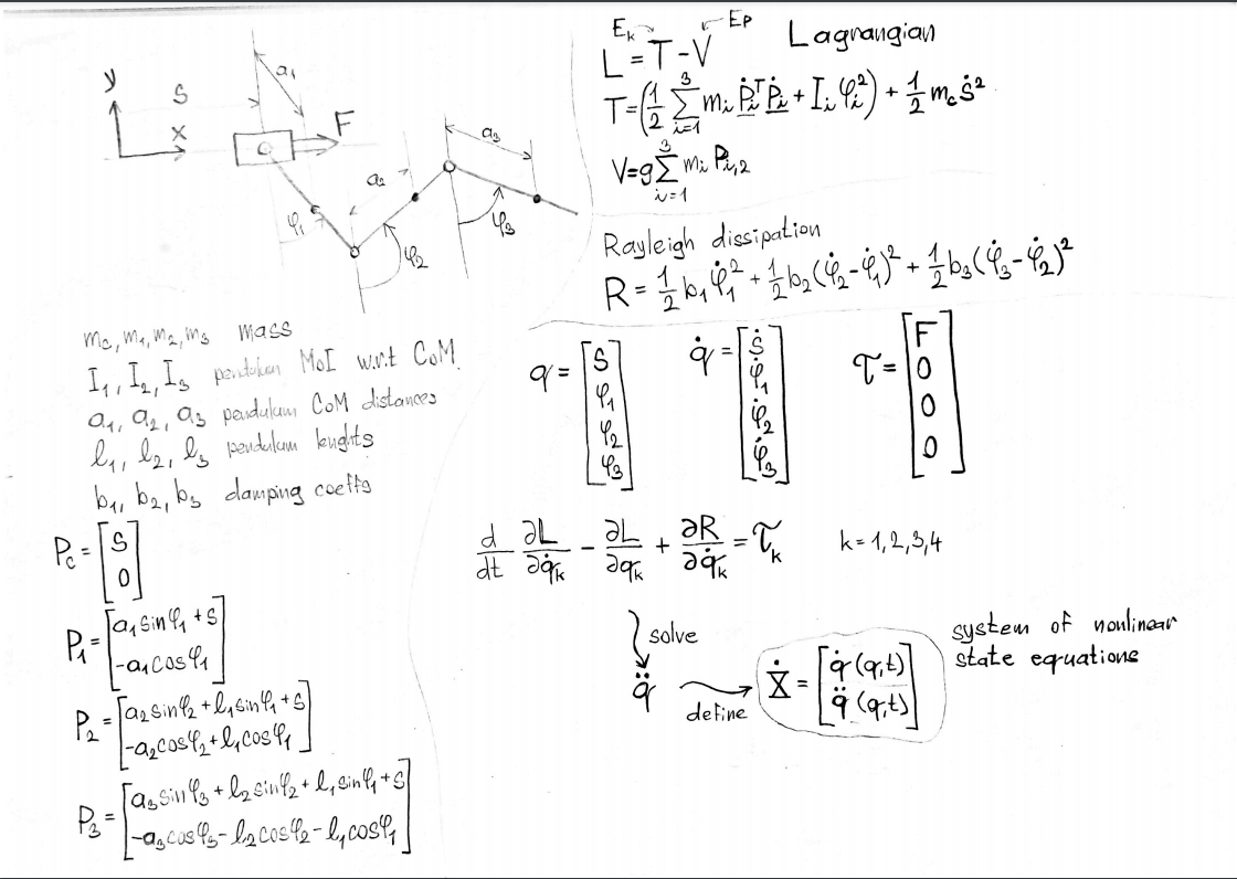
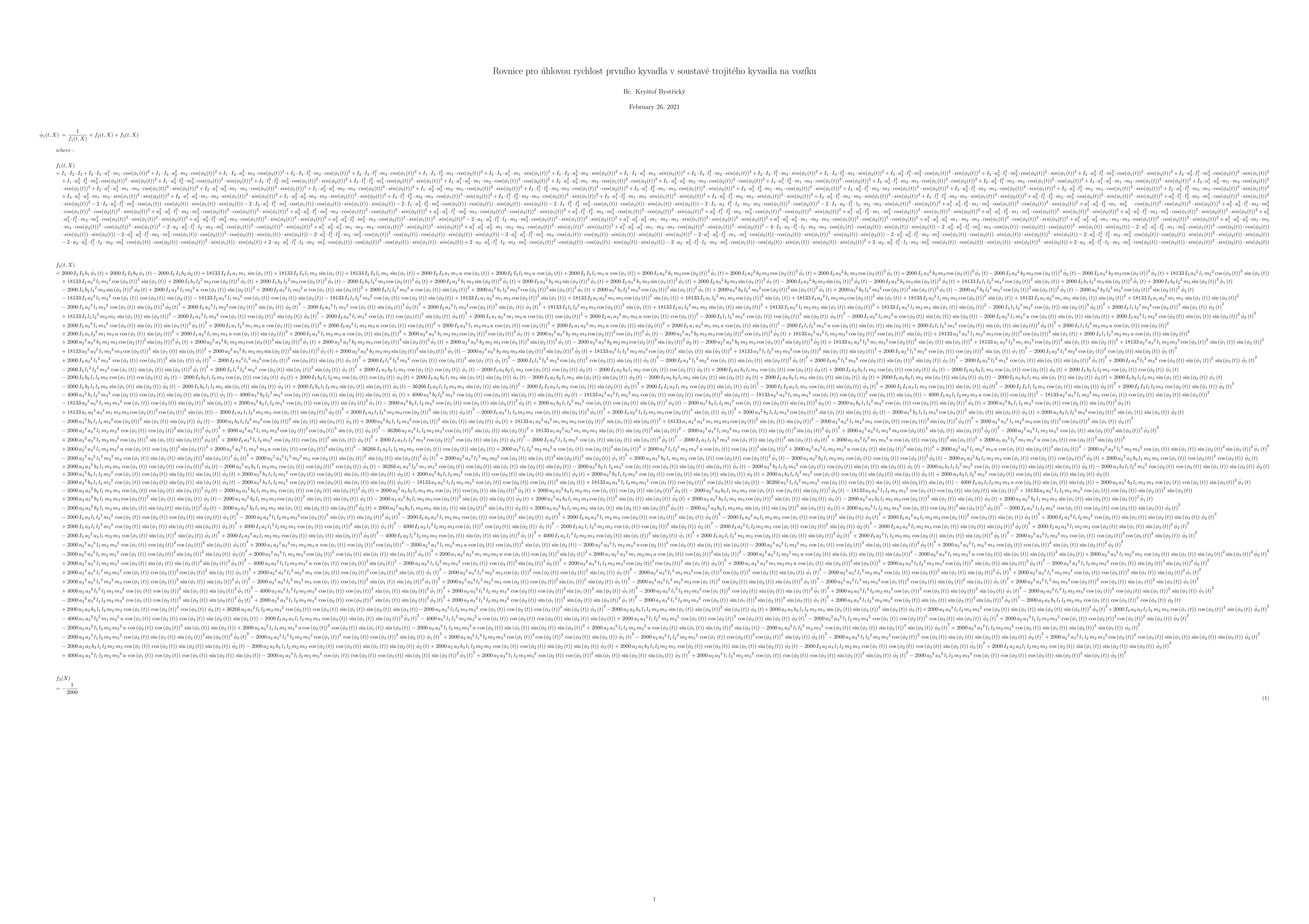
Simulation of the pendulum-cart system https://user-images.githubusercontent.com/55796835/127646378-228cc491-b344-4ab0-9caf-d83239d9fb81.mp4

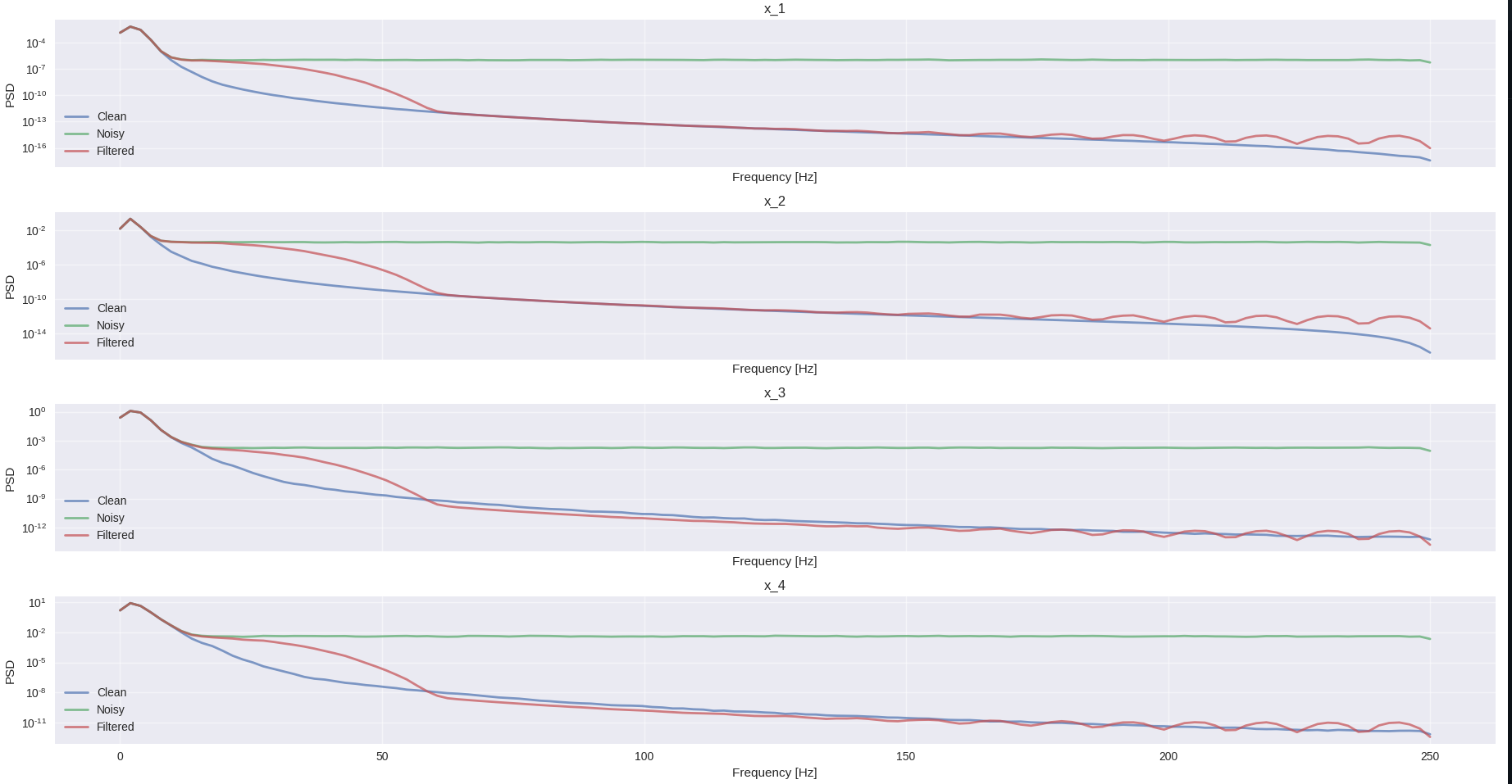
Simulation of the reference pendulum-cart model and model identified using SINDy from noisy data. https://user-images.githubusercontent.com/55796835/127749887-452fa243-7efa-4761-86bd-0d9dca009ddb.mp4

Reference model vs Bootstrapped model https://user-images.githubusercontent.com/55796835/127749898-489bcebc-fb2e-4f7f-bea3-ada7994ee317.mp4

SINDy model vs Bootstrapped model https://user-images.githubusercontent.com/55796835/127749894-e9e21523-7ae3-4ad0-b916-287db34bbfc4.mp4

Lorenz reference vs identified, nonlinear and discontinuous input sgn(u1) to dx1 https://user-images.githubusercontent.com/55796835/127779031-6db32467-f23b-4574-8389-3a0982e1bd85.mp4

Model identified from real measurement data https://user-images.githubusercontent.com/55796835/127922658-35e7b487-f04e-431a-a6e0-aed10cce4e76.mp4

The real measurement data, visualized https://user-images.githubusercontent.com/55796835/127937959-67bdb377-eedd-4c89-b2cd-edfd253517ce.mp4

sindy's People

Contributors

bystrickyk avatar

Stargazers

 avatar  avatar  avatar  avatar  avatar  avatar  avatar  avatar

Watchers

 avatar  avatar

sindy's Issues

Double pendulum cart, but with a good function library

Trig functions of double angle differences can be decomposed into sine and cosine monomials like this:
image

Using completely clean data, acceleration measurements generated using the analytical model (rather than numerical differentiation)

Discovered models, dotx4 = cart acceleration, dotx5 = first pendulum angular acceleration, dotx6 = second pendulum angular acceleration
4
5
6

Prediction results:
Figure_4
Figure_5
Figure_6

Prediction is nearly perfect, but simulated trajectories decouple immediately; it might be due to a bug in the code though
https://user-images.githubusercontent.com/55796835/117227428-11243b00-ae17-11eb-9df1-95b025d6f23b.mp4

Cart+Pendulum, Identification from measurements

Forcing signal extremely noisy - must be filtered
image

Acceleration predictions
image

Symbolic equations for the chosen models:
image
The cart acceleration is apparently exploding because of the denominator constant term being smaller than the cos^2 term.

Models:
image

Function library

The dynamics of multiple pendulum systems are described by trigonometric functions, the function library (~regression matrix) must therefore contain trigonometric functions for successful model identification. The trigonometric terms for a double pendulum look like this:
image
The library has to contain sine/cosine functions of many different pendulum angle sums. First, I create the angle sum signals; I multiply the angles by numbers from -2 to 2 and then create all possible sums (combinations). These sum angle signals are then used for calculating the respective sine/cosine signals. The resulting trigonometric signals for a double pendulum system look like this:
image
where x[2] and x[3] are the angles of the first and second pendulums.
This crude way of producing trigonometric functions creates one major problem. Two different angle sums inside a trigonometric function might create perfectly correlated signals because of the oddness/evenness of trigonometric functions. For example, the signals sin(x1 - 2x2) will be perfectly negatively correlated with sin(-x1 + 2x2). The presence of perfectly correlated regressors is a problem, because it creates ambiguity and trivial solutions (when LHS is guessed as a term that has a perfectly correlated term in the library, the RHS is just the twin term).
One way to solve this is to create the angle sums with the oddness/evenness problem in mind - this requires manually specifying the sum rules and lengthy IF statements to make sure no "twin" angle sum is created. I attempted this at first, but it gets quite complicated and convoluted when working with 3 or more angles. I thought of re-defining the trigonometric functions into complex exponential functions using Euler's formula, as the problem might be easier to deal with in the exponential formulation, but I found a "dumber", simpler, engineer's solution.
A simpler way to remove twin terms is to create the trig functions by all angle sum combinations just as before, and then calculating a huge correlation matrix and removing all signals that have a 1 or -1 in the lower triangular part of the correlation matrix. This method of removing twin signals scales well for any number of angles and doesn't require as much mathematical rigor.

Correlation matrix of trigonometric terms for a triple pendulum:
full_identities
Note the two "lines" crossing the main diagonal, one black (all -1 values) and one yellow (all 1 values), these indicate twin coupling between the two signals. The axis labels are supposed to be signal labels describing the regressor, but they're overlapping. Here's a picture zoomed on the upper line crossing of the main diagonal:
zoom_identities

Removing these problematic twin terms and calculating the correlation matrix again results in a diagonally dominant correlation matrix. Here's the correlation matrix after removing all terms that were -1 or 1 on the lower triangular (excluding main diagonal) correlation matrix:
full_no_identities
zoom_no_identities

Full single pendulum

In this model, u specifies the force on the cart. The equations dx3/dt and dx4/dt in this case are rational. Equations dx1/dt and dx2/dt are equal to x3 and x4 respectively.
image
The equations are then rewritten into an implicit form and each equation is identified separately.

I constructed the function library to contain the relevant functions from the implicit dynamics. Of course, in practice, the actual implicit dynamics would be unknown, I'm doing this merely for testing purposes. The correlation matrix of the full library:
corrmat
Note that while there are some perfect correlations, the full library is reduced for each equation identification. For example, if our goal was to identify the equation dx_3 / dt, we'd remove all the terms from the library that contain any other dx_i / dt. This way, the annoyance of poorly conditioned regression is partly omitted.

Solutions as implicit models for each equation dx_i / dt. The columns are the regressor parameters and the rows are the identified equations, with description of the LHS guess, the equation's fit to training data and the model's index:
1617359354_4896944_implicit_sols
1617359358_3707457_implicit_sols
1617359361_469719_implicit_sols
1617359368_793456_implicit_sols

Simulation of the identified model next to the analytical model used for training data generation. When constructing the full model from the identified equation, the equations with the best fits were picked:
https://user-images.githubusercontent.com/55796835/113409524-c21b5e00-93b1-11eb-8a7f-8f266dc609fd.mp4

Decomposing the implicit equation for dx3 / dt into terms:
dx_3_terms

Some of the terms have relatively very little energy. This might mean that some terms are dominant, and some are less pronounced or only pronounced in specific conditions - gathering testing data in those conditions would be beneficial for more accurate model. For example, if the forcing is too weak, the pendulum never gets to the upper position and therefore there's no information about the dynamics around the unstable singularity state-space point, which is very important in the actual dynamics.

Numerical differentiation and noise filtering

Numerical differentiation decreases the Signal/Noise Ratio (SNR), and the measured data (position of the cart and the angle of the endulum) must be differentiated twice (to obtain velocity and acceleration). This means there's a need for robust pre-processing filtering step. Normal kernel-based filters probably aren't good enough and I'd like to use FFT, so I'll do part of the filtering by cutting off higher frequencies. The cutoff frequency will be based off of the PSD of each signal. Coincidentally, I found a paper ( https://arxiv.org/abs/2009.01911 ) again from UW, which finds the cutoff frequency similarly and has the same co-author (prof. Kutz) as the SINDy paper.

PSD of the state signals, the 'Filtered' signal is filtered with a non-causal flattop kernel with the size 60. Real measurements will contain only measurements x1 and x2, x3 and x4 must be gotten through differentiating them.
image

Mathematical model of a multiple pendulum/cart system

Definition of the Lagrangian and Rayleigh dissipation. The Lagrangian along with the Rayleigh dissipation function are then rewritten into MATLAB, where the system's Lagrange equations are analytically solved and transformed into state-space form.
lagrang

Resulting equations for the angular accelerations of the pendulums are massive. Here is the ODE describing the acceleration of the first pendulum (there's a mistake, Phi_1 on the left hand side should have two dots instead of one):
eqns

The analytical state-space derivative equations are then automatically rewritten into MATLAB ODE functions, so they can be numerically solved in time. A little manual adjustment has to be done to the MATLAB ODE functions to define the system input (cart acceleration) as a time-variant function, so the system can be simulated with external input forcing. The system parameters are then guessed, and the system is simulated and animated to visually verify the model.

No forcing:
animH

With forcing, input signal is set as a random walk signal (although it's constrained, so the cart doesn't move too far from 0 and to make sure the cart acceleration is below ~4G):
https://user-images.githubusercontent.com/55796835/109891105-c3f5e280-7c88-11eb-9492-7fb70c044870.mp4

I also simplified the model by removing two of the pendulums, the state equations are much smaller and therefore better for testing the identification method.
https://user-images.githubusercontent.com/55796835/109821129-f62a2480-7c35-11eb-84bc-1b48f13ad1b2.mp4

Single pendulum on a cart - Identification results

Analytical model with all physical parameters = 1
image

State data X was generated by a numerical simulation of an analytically derived model. State derivatives dX (dot X) were computed from state data X using spectral differentiation. Other nonlinear functions were constructed from these signals.

The function library A (regression matrix) signals A_col (regressors) look as follows:
sim_data

Correlation matrix of the function library:
theta_corr

The goal of regression is to find sparse right-hand side solution (x) to a left-hand side guess term (b). There's only one regression hyperparameter - the threshold. For each LHS guess term, the regression is repeated many times for different threshold values. Nonzero, unique solutions are then saved for future comparison and modelling.

After trying all the possible LHS guess terms and solving the regression problems, we're left with a set of implicit equations that are candidates for equations describing the system dynamics. If two particular terms are in the real dynamics, each one of those should generate a solution if used as a LHS guess. We can use this fact to look at all the models and pick the models which contain the same active terms.

Each model equation is described by a vector of parameters and the corresponding term. The identified implicit equations are below, each row is a separate model. The labels on the left are in the form "{LHS term guess | model index}:
implicit_eqns_raw

For each model, I calculate an activation vector, that describes which parameters are non-zero, or which terms were identified as active in the model. Non-zero elements of the original solution vector become 1, others stay 0:
active_terms

We can then compare different models by calculating the L1 distance between their activation vectors. An activation distanceof 0 means that the models contain exactly the same terms, although their actual parameters will be almost always different, because the equations are implicit. An activation distance of 1 means the models differ by one term, and so on...

Matrix of activation distances between identified implicit equations:
activation_dist

The labels for each distance matrix element contain two parts, the left one is the LHS guess and the right one is the model index. Activation distances on the diagonal are all 0, because each model is identical to itself. The matrix is symmetrical, so we can focus only on the lower triangular part. We can for example see that model 8 (with a LHS guess of dX4) contains the same parameters as model 5. These models are therefore good candidates for equations describing the implicit dynamics.

Implicit models, normalized so that the smallest parameter is 1 or -1, so that the model parameters can be directly compared:
implicit_eqns

We can see that the implicit equations 5, 8 and 17 are nearly identical. These equations accurately describe the implicit form of the state equation for dX4. Note that it could also be used for calculating dX3, the simulation model was however defined so that dX3 = u, and the input signal u was removed from the function library, because it was perfectly correlated to dX3 and therefore would make the regression ill-conditioned.

Here are the results if input signal u is included in the function library:
Correlation matrix:
theta_corr_with_u
Activation distance matrix:
activation_dist_poorcond
Implicit solutions:
implicit_eqns_raw_poorcond
It seems that the correct implicit equation was also identified (models 20, 10, 7).
The positions of x-axis labels for larger trig functions might be confusing, I'll rotate them so they're vertical next time.

Recommend Projects

  • React photo React

    A declarative, efficient, and flexible JavaScript library for building user interfaces.

  • Vue.js photo Vue.js

    ๐Ÿ–– Vue.js is a progressive, incrementally-adoptable JavaScript framework for building UI on the web.

  • Typescript photo Typescript

    TypeScript is a superset of JavaScript that compiles to clean JavaScript output.

  • TensorFlow photo TensorFlow

    An Open Source Machine Learning Framework for Everyone

  • Django photo Django

    The Web framework for perfectionists with deadlines.

  • D3 photo D3

    Bring data to life with SVG, Canvas and HTML. ๐Ÿ“Š๐Ÿ“ˆ๐ŸŽ‰

Recommend Topics

  • javascript

    JavaScript (JS) is a lightweight interpreted programming language with first-class functions.

  • web

    Some thing interesting about web. New door for the world.

  • server

    A server is a program made to process requests and deliver data to clients.

  • Machine learning

    Machine learning is a way of modeling and interpreting data that allows a piece of software to respond intelligently.

  • Game

    Some thing interesting about game, make everyone happy.

Recommend Org

  • Facebook photo Facebook

    We are working to build community through open source technology. NB: members must have two-factor auth.

  • Microsoft photo Microsoft

    Open source projects and samples from Microsoft.

  • Google photo Google

    Google โค๏ธ Open Source for everyone.

  • D3 photo D3

    Data-Driven Documents codes.