Machine Learning (CS-GY6923) Final Project

This repository and project was developed for the graduate level machine learning class CS-GY-6923 at NYU. The class professor is Linda Sellie.

The author of the project is Justin Snider.

Introduction

In this project we implements three extensions to the basic neural network machine learning strategies introduce in the class. For each extension we demonstrate how the strategy can be implemented using the libraries scikit-learn and PyTorch. Then, we will implement the strategy ourselves using only NumPy.

The first extension we develop is convolution layers. Second, we build on CNN to introduce the use of pooling. For the final extension we introduce the use of skip links.

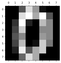
We use two datasets to evaluate the performance of our code. First, we use the SciKit Hand Written Digits used in class. This dataset has 10 classes, which are the digits 0 through 9. There are 1,797 sample. Each sample is in the format of an 8 x 8 pixel grid. The original source of the data used by SciKit is the UCI Machine Learnign Respository. Here we have an example of a zero from the dataset.

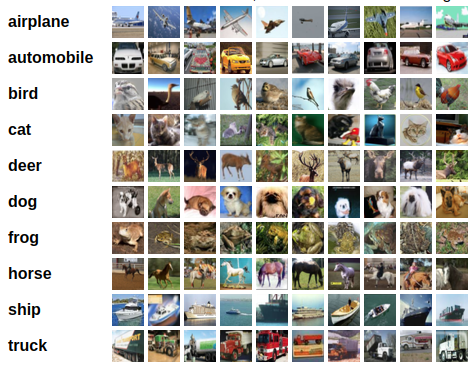
The second dataset is the more challenging CIFAR-10 . We again have 10 classes. There are 60,000 total images, with 6,000 images per class. However, for the sake of efficiency we use just 1,000 images randomly selected. The images are formated as 32 x 32 pixels with 3 color channels. Here we have an example of 10 images from each of the 10 classes.

Required Setup

Just click on the links provided in this guide and you are ready to go!

Inside each of the live Google Colab notebooks code is provided to allow you to mount Your Google Drive and load the data used to a 'temp-data' inside the root 'My Drive' folder. The data downloaded included is a limited and compressed portion of the MNIST and CIFAR-10 datasets. When you are done running these notebooks you can simply delete the 'temp-data' folder from Google Drive to recover the space.

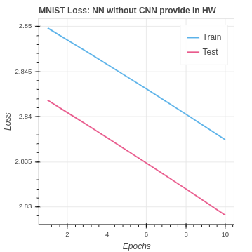
Benchmarks Neural Network Without Extension

For consistency sake, we use the same training and test sets for all the tests. In addition, we visualize the first 10 epochs of all tests in the same manner. You will find for all the successful code sets included a visualization of the loss, the accuracy, and the accuracy against the benchmark.

Using the interactive graphs in the live Google Colabs notebook you can get all the specific value by hovering your mouse over the point you want to investigate.

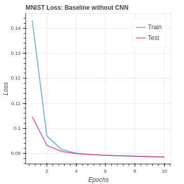
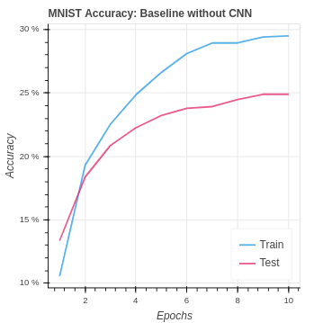
Our naive baseline will be a PyTorch Neural network without extension. The baseline is built using the same architecture as the neural network introduced in Homework 08. The input layer is set by the number of input values for the given dataset. The hidden layer has 30 nodes. The output layer is set by the number of classes to predict, which is 10 for both of our datasets. The non-linear activation for the hidden and output layers is the sigmoid function.

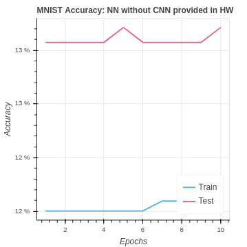
We have the following baseline performance for our naive neural network on the MNIST dataset.

To establish a better MNIST baseline we created a PyTorch Neural network using the same 8 x 8 pixel dataset. Here is the custom PyTorch dataset class code:

class MNISTDataset(Dataset):
    def __init__(self, data, label):
        self.data = data.reshape((-1,8,8,1))
        self.label = label

    def __len__(self):
        return len(self.label)

    def __getitem__(self, item):

        # swap color axis because
        # numpy image: H x W x C
        # torch image: C X H X W
        image = self.data[item].transpose((2, 0, 1))
        image = torch.from_numpy(image)
        target = self.label[item]
        target = torch.from_numpy(target)
        return (image, target)

Our PyTorch Neural Network class uses the same neural network structure with 64 input nodes, 30 hidden nodes, and 10 output nodes. In addition, we use the same sigmoid activation as the original homework assignment code. Here is the Neural Network class:

class MNIST(nn.Module):
    # Our batch shape for input x is (1, 8, 8)
    def __init__(self):
        super(MNIST, self).__init__()
        self.fc1 = nn.Linear(64, 30)
        self.fc2 = nn.Linear(30, 10)

    def forward(self, x):
        x = x.view(-1, 8 * 8)
        x = torch.sigmoid(self.fc1(x))
        x = torch.sigmoid(self.fc2(x))
        return x

We optimized the hyper-parameters and used the following:

Hyper-parameter	Value
batch size	1
learning rate	0.01
epochs	10

We have the following baseline performance for our naive neural network on the MNIST dataset.

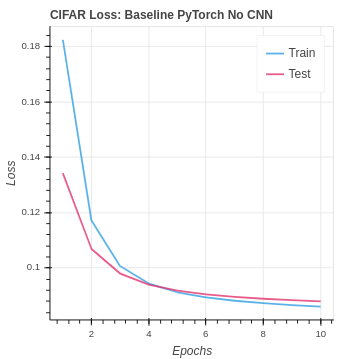
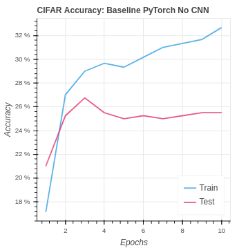
The CIFAR baseline set up is very similar for the MNIST baseline naive neural network. We changed the network architecture to accommodate the larger input image size and additional channels.

Baseline Synopsis

Algorithm	Training Set Accuracy	Test Set Accuracy
MNIST Baseline No CNN	29.50%	24.90%
CIFAR Baseline No CNN	32.67%	25.25%

As you will see later in the report the PyTorch extension implementations do better than the NumPy extension implementations. I was concerned that my extension implementations had errors. So I found two implementations by other of the extension in NumPy. Plugging in our datasets the performance on both of the NumPy extensions be others was actually similar or worse than the results achieved. There is no room in this report for comparison due to the two page per extension limit. In addition, the assignment did not require the information. As a result, I did not include the statistics here. However, I would like to note I have verified that the NumPy performance on these extensions is in line with the performance by code published by others.

For all of the reasons above it is notable that our baseline build in PyTorch has an advantage over our NumPy implementations from the start. In addition, our PyTorch with extension implementations also have an advantage over the NumPy implementations.

Extension 01 // Neural Network with Convolution

Convolutional neural networks are often used to evaluate visual imagery. So given our challenge using the MNIST and CIFAR-10 input images to predict their class the development of a CNN is a worthy extension of our baseline neural network.

The convolution will need to have a set of kernels, also called filters, that multiplied against the input data on the forward pass to create the output maps. On the backward pass the derivatives multiplied by the input values are used to update each kernel. Ideally, in the end we have a filter that will better help us predict the correct class on the next round.

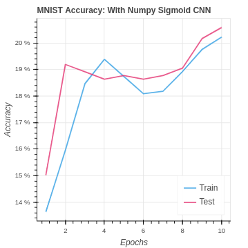
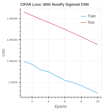
Extension 01 // Neural Network with Convolution // Using NumPy

We first develop CNN using NumPy exclusively. For consistency, we start with the same sigmoid activation and after the convolution layer, we use a similar fully connected set of layers to what is in the naive baseline setup. However, we have gone from 64 inputs to the fully connected layer up to 6 * 6 * 64. Although we are using CNN to find new relationships in the data the signal is being lost. Our performance is terrible. We are doing worse than the baseline and worse than just guessing the mode class every time. In addition, our models get worse with training.

In NumPy we develop a CNN class. The class will carry out initialization, forward propagation, and backwards propagation.

class CNN:

    def __init__(self, num_kernels, pool_size, out_nodes, seed):
        self.kernels = self.Kernels(num_kernels)  # 8x8x1  to 6x6x10
        self.sigmoid = self.Sigmoid(6 * 6 * num_kernels, out_nodes)  # 6x6x10 to 10
        np.random.seed(seed)

    class Kernels:
        # The set of kernels and kernel functions

        def __init__(self, num_kernels):
            self.num_kernels = num_kernels
            self.size_kernel = 3
            self.kernels = np.random.randn(num_kernels, 3, 3) / (self.size_kernel ** 2)

        def forward(self, x):
            self.cur_x = x

            height, width = x.shape
            result = np.zeros((height - 2, width - 2, self.num_kernels))

            for i in range(height-2):
                for j in range(width-2):
                    block = x[i:(i+3), j:(j+3)]
                    result[i,j] = np.sum(block * self.kernels, axis=(1, 2))
            return result

        def back(self, delta_cnn, alpha):
            height, width = self.cur_x.shape
            dk = np.zeros(self.kernels.shape)
            delta_cnn = delta_cnn.reshape(height-2, width-2,self.num_kernels)
            for i in range(height - 2):
                for j in range(width - 2):
                    block_x = self.cur_x[i:(i+3), j:(j+3)]
                    # block_delta = delta_cnn[i:(i+3), j:(j+3)]
                    for k in range(self.num_kernels):
                        dk[k] += delta_cnn[i,j,k] * block_x
            self.kernels += -alpha * dk

    class Sigmoid:
        # Use a fully connected layer using sigmoid activation

        def __init__(self, in_nodes, out_nodes):
            self.w = np.random.randn(out_nodes, in_nodes) / in_nodes
            self.b = np.zeros((out_nodes, 1))

        def sig(self,z):
            return 1 / (1+np.exp(-z))

        def d_sig(self,z):
            return self.sig(z) * (1-self.sig(z))

        def loss(self, y, yhat):
            self.y_vector = np.zeros((len(yhat), 1))
            self.y_vector[y, 0] = 1.0
            loss = np.linalg.norm(self.y_vector - yhat)
            accuracy = 1 if np.argmax(yhat[:, 0]) == y else 0
            return loss, accuracy

        def forward(self, x):
            # TODO forward pass
            self.z_cnn = x.reshape(-1, 1)
            self.a_cnn = self.sig(self.z_cnn)

            self.z_out = np.matmul(self.w, self.a_cnn) + self.b
            self.a_out = self.sig(self.z_out)

            return self.a_out

        def back(self, alpha):

            w_grad = np.zeros(self.w.shape)
            b_grad = np.zeros(self.b.shape)

            # get delta for out layer
            delta_out = -(self.y_vector - self.a_out) * self.d_sig(self.z_out)

            # get delta for hidden layer
            delta_pool = np.dot(self.w.T, delta_out) * self.d_sig(self.z_cnn)

            w_grad += -alpha * np.matmul(delta_out, self.a_cnn.T)
            b_grad += -alpha * delta_out
            # TODO back pass through pool and cnn layers
            return delta_pool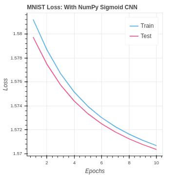

We find that performance is not very good in comparison with our baseline neural network that achieved around 45% testing accuracy. Our performance on the CIFAR-10 dataset is even worse.

We experimented with several possible solutions including alternate different hidden node counts, additional hidden layers, different numbers of kernels, and other dead-end ideas. In the end, the most effective solution is to change the activation function. Simply writing an alternative class using leaky ReLu for the activation gives a great performance as you can see below.

Here is the new ReLu class:

    class ReLu:
        # Use a fully connected layer using sigmoid activation

        def __init__(self, in_nodes, out_nodes):
            self.w = np.random.randn(out_nodes, in_nodes) / in_nodes
            self.b = np.zeros((out_nodes, 1))
            self.y_vector = np.zeros((1))
            self.z_cnn = np.zeros((1))
            self.a_cnn = np.zeros((1))
            self.z_out = np.zeros((1))
            self.a_out = np.zeros((1))

        def f(self, z):
            return np.where(z > 0, z, z * 0.2)

        def d_f(self, z):
            test = np.where(z>0, 1.0, 0.2)
            return np.where(z>0, 1.0, 0.2)

        def sig(self, z):
            return 1 / (1 + np.exp(-z))

        def d_sig(self, z):
            return self.sig(z) * (1 - self.sig(z))

        def loss(self, y, yhat):
            self.y_vector = np.zeros((len(yhat), 1))
            self.y_vector[y, 0] = 1.0
            loss = np.linalg.norm(self.y_vector - yhat)
            accuracy = 1 if np.argmax(yhat[:, 0]) == y else 0
            return loss, accuracy

        def forward(self, x):
            # In Shape: (16, 16, 18)
            self.z_cnn = x.reshape(-1, 1)
            # Reshape: (4608, 1)
            self.a_cnn = self.f(self.z_cnn)

            self.z_out = np.matmul(self.w, self.a_cnn) + self.b
            # Product Shape: (10,1)
            self.a_out = self.f(self.z_out)

            # Out Shape: (10,1)
            return self.a_out

        def back(self, alpha):

            w_grad = np.zeros(self.w.shape)
            b_grad = np.zeros(self.b.shape)

            # get delta for out layer
            delta_out = -(self.y_vector - self.a_out) * self.d_f(self.z_out)

            # get delta for hidden layer
            delta_pool = np.dot(self.w.T, delta_out) * self.d_f(self.z_cnn)

            w_grad += -alpha * np.matmul(delta_out, self.a_cnn.T)
            b_grad += -alpha * delta_out

            return delta_pool

We have the added bonus that ReLu is computationally simpler, using less time and less resources. Here are the great results we achieved primarily be going from sigmoid to Leaky ReLu on both the MNIST and CIFAR-10 datasets.

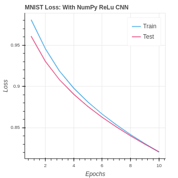
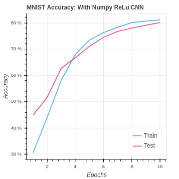
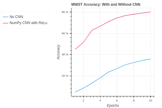
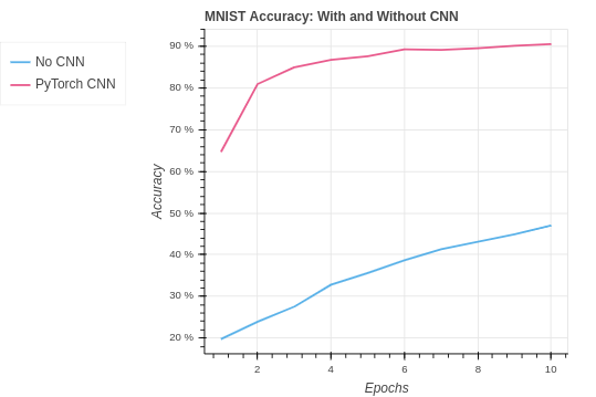
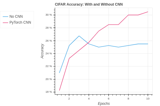
Finally, lets take a look at our NumPy CNN compared with the baseline performance. Our CNN does very well with the MNIST dataset essentially doubling our accuracy.

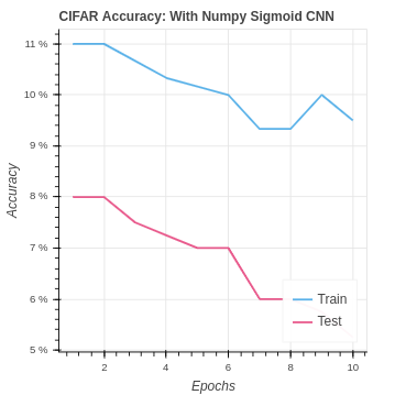
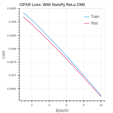
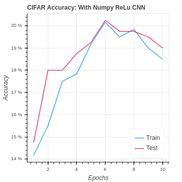
The story is different with the CIFAR dataset. Our simplistic CNN is overwhelmed by the larger number of pixels and the 3 color channels. Fortunately our PyTorch CNN does do better than the baseline. But it is clear the NumPy is not doing well. This is likely a result of our relatively naive implementation of CNN that does not make any extra moves to optimize or add stability as is done with PyTorch. You can see this better PyTorch performance in the next section.

Extension 01 // Neural Network with Convolution // Using PyTorch

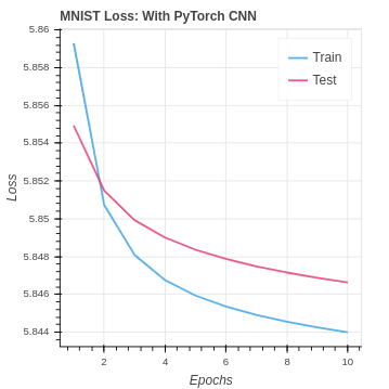
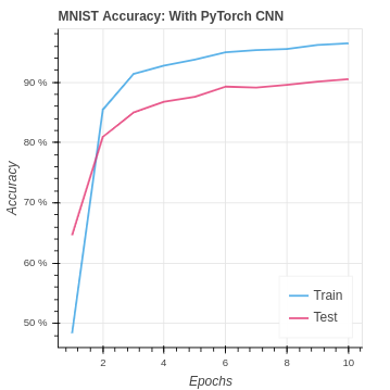
We will be using the following function to apply convolutions: torch.nn.Conv2d* (in_channels, out_channels, kernel_size, stride, padding). The function applies a 2-D convolution over an input signal composed of several input planes. Using PyTorch to construct our CNN we were able to greatly increase our performance over both the baseline neural network and the NumPy CNN implementation on the MNIST dataset.

Both the convolution and fully connected layer functions in PyTorch or modified from the naive equations we implement in NumPy. The modification stabilizes the values passing through the network. The inevitable rounding off of large and small values caused us to lose the potential effectiveness of CNN in our NumPy implementation. However, in PyTorch, our test set accuracy moves from the baseline of under 50% up to over 90% on the MNIST dataset.

You can see the PyTorch functions and their implementation explanations in the PyTorch documentation here.

We first implement a dataset class for use with MNIST.

class MNISTDataset(Dataset):
    def __init__(self, data, label):
        self.data = data.reshape((-1,8,8,1))
        self.label = label

    def __len__(self):
        return len(self.label)

    def __getitem__(self, item):

        # swap color axis because
        # numpy image: H x W x C
        # torch image: C X H X W
        image = self.data[item].transpose((2, 0, 1))
        image = torch.from_numpy(image)
        target = self.label[item]
        target = torch.from_numpy(target)
        return (image, target)

Our new neural network model implements the use of a convolution layer.

class MNIST(nn.Module):

    # Our batch shape for input x is (1, 8, 8)

    def __init__(self):
        super(MNIST, self).__init__()

        # Input channels = 1, output channels = 18
        self.conv1 = torch.nn.Conv2d(1, 18, kernel_size=3, stride=1, padding=1)
        # self.pool = torch.nn.MaxPool2d(kernel_size=2, stride=2, padding=0)

        self.fc1 = nn.Linear(18 * 8 * 8, 64)
        self.fc2 = nn.Linear(64, 10)

    def forward(self, x):

        x = F.relu(self.conv1(x))
        x = x.view(-1, 18 * 8 * 8)
        x = torch.sigmoid(self.fc1(x))
        x = self.fc2(x)
        x = F.log_softmax(x, dim=1)

        return x

Using PyTorch to construct our CNN we were able to greatly increase our performance over both the baseline neural network and the NumPy CNN implementation on the MNIST dataset.

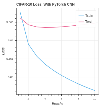
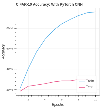
We are able to do better than the baseline on the CIFAR-10 dataset. However, you can see we are overfitting the training set in the extreme. As the input data size grows, the training set remains small, and the classes become more difficult to identify over-training is, unfortunately, the natural result.

A good follow up would be to explore ways of reducing over-fitting. By using an architecture with pooling and skip links we can improve the performance and reduce the over-training. We will explore these two directions in the next two notebooks. In addition, using more training data, more layers, and a variety of kernel sizes would all help as well and would be worthy of further experimentation.

Extension 01 // Synopsis

Algorithm	Training Set Accuracy	Test Set Accuracy
MNIST Baseline No CNN	29.50%	24.90%
MNIST Sigmoid NumPy CNN	20.22%	20.58%
MNIST Leaky ReLu NumPy CNN	81.17%	80.11%
MNIST PyTorch with CNN	96.47%	90.54%
CIFAR Baseline No CNN	32.67%	25.25%
CIFAR Sigmoid NumPy CNN	9.5%	5.25%
CIFAR Leaky ReLu NumPy CNN	18.5%	19.00%
CIFAR PyTorch CNN	96.00%	30.50%

Extension 02 // Pooling

We use our CNN from extension 01 as a starting point. Pooling is traditionally applied to the output map a convolution before activation. Pooling can come in many flavors including max pooling, average pooling, and several other less common strategies. Pooling can be applied to reduce the size of an output map, while keeping the number of channels remains the same. Inversely, pooling can keep the output map the same size, but reduce number of channels.

Extension 02 // Neural Network with Pooling // Using NumPy

To implement pooling we must revise our CNN class to include a Pooling CNN. In addition, we also modify our ReLu class to respond the reduced size output of the pooling layer.

    class Pool:
        # use max pooling with size 2x2
        def __init__(self, pool_size):
            self.dim = pool_size  # size of the pool
            self.cur_pool_input = np.zeros((1))

        def forward(self, x):
            self.cur_pool_input = x
            height, width, num_k = x.shape
            result = np.zeros((height // self.dim, width // self.dim, num_k))
            for i in range(height // self.dim):
                for j in range(width // self.dim):
                    block = x[(i*self.dim):(i*self.dim+self.dim), (j*self.dim):(j*self.dim+self.dim)]
                    result[i,j] = np.amax(block, axis=(0,1))
            return result

        def back(self, delta_pool):
            height, width, num_k = self.cur_pool_input.shape
            delta_pool = delta_pool.reshape((height//2, width//2, num_k))
            delta_cnn = np.zeros((height, width, num_k))

            for i in range(height // self.dim):
                for j in range(width // self.dim):
                    block = self.cur_pool_input[(i*self.dim):(i*self.dim+self.dim),(j*self.dim):(j*self.dim+self.dim)]
                    b_h, b_w, b_k = block.shape
                    maximum = np.amax(block, axis=(0,1))
                    for s in range(b_h):
                        for t in range(b_w):
                            for u in range(b_k):
                                if block[s, t, u] == maximum[u]:
                                    delta_cnn[i*2+s, j*2+t, u] = delta_pool[i,j,u]
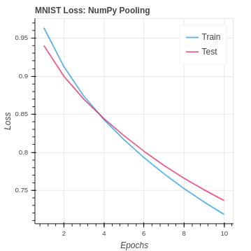
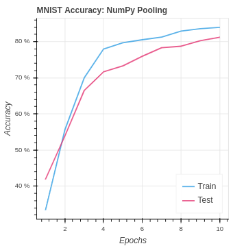
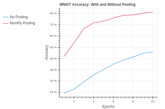
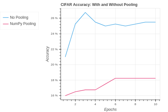
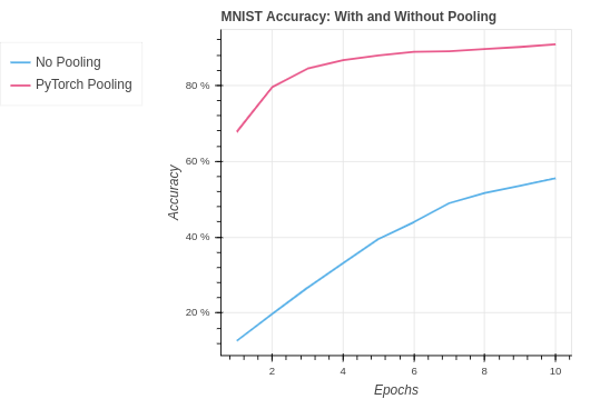
            return delta_cnn

On the MNIST dataset our performance is an improvement. However, it is notable that a pooling layer actually reduces the amount of information in the model. For this reason we can see our performance is very similar to the NumPy CNN without pooling.

In ResNet they do not use pooling to avoid the loss if signal in the network. Instead they use a kernel with a stride of 2 to shift the size of the model.[7] In addition, they add more layers to the model whenever using the stride of 2. This provides a way to for the signal to persist.

Extension 02 // Neural Network with Pooling // Using PyTorch

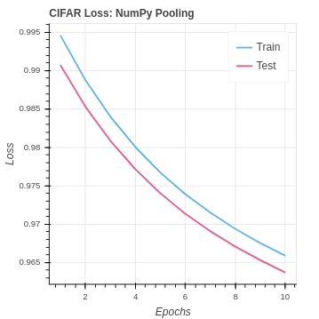
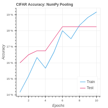
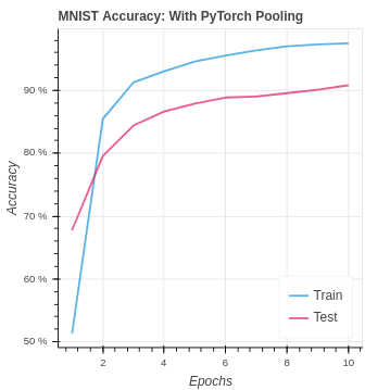
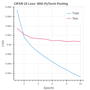
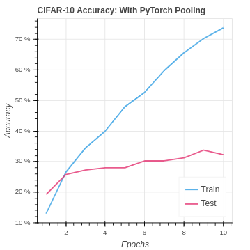
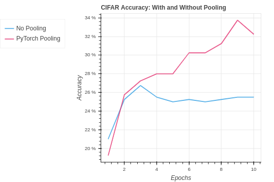
To implement pooling in PyTorch we use the function $torch.nn.MaxPool2d(kernel_size, stride, padding)$ Here is our new neural network class using the pooling function on our MNIST class. There is a similar implementation for the CIFAR-10 dataset.

Again we see the results are quite similar to the PyTorch CNN implementation without pooling. In the CIFAR-10 version, we are seeing a slightly better test set performance. This suggests the pooling may be helping the model to generalize better to the test set. However, the impact in the case is very weak.

Although we have not improved our model over the PyTorch CNN without pooling we are still getting the same performance. So we are doing better than the baseline neural network.

class MNIST(nn.Module):

    # Our batch shape for input x is (1, 8, 8)

    def __init__(self):
        super(MNIST, self).__init__()

        # Input channels = 1, output channels = 18
        self.conv1 = torch.nn.Conv2d(1, 18, kernel_size=3, stride=1, padding=1)
        self.pool = torch.nn.MaxPool2d(kernel_size=2, stride=2, padding=0)
        self.fc1 = torch.nn.Linear(18 * 4 * 4, 64)
        self.fc2 = torch.nn.Linear(64, 10)

    def forward(self, x):

        x = F.relu(self.pool(self.conv1(x)))
        x = x.view(-1, 18 * 4 * 4)
        x = self.fc1(x)
        x = torch.relu(x)
        x = self.fc2(x)
        x = F.log_softmax(x, dim=1)

        return x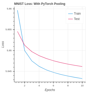

Extension 02 // Synopsis

Algorithm	Training Set Accuracy	Test Set Accuracy
MNIST Baseline No Pooling	29.50%	24.90%
MNIST NumPy Pooling	83.95%	81.22%
MNIST PyTorch Pooling	97.50%	90.82%
CIFAR Baseline No Pooling	32.67%	25.25%
CIFAR NumPy Pooling	19.17%	18.25%
CIFAR PyTorch Pooling	73.83%	32.25

Extension 03 // Neural Networks with Skip Links

It has been shown that an effective technique for improving neural networks for some applications is to increase the number of layers as shown in the paper by the creators of ResNet.[7] The group was able to a series of competitions with different applications setting new high-water benchmarks. The intuition says both forward propagation and back propagation signals die off in deep neural networks. However, if we can find a way to allow the signal to persist we can make deep neural networks a powerful learner and predictor.

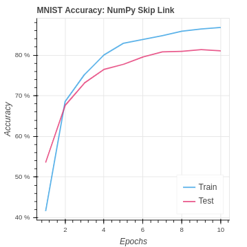
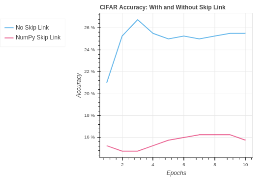
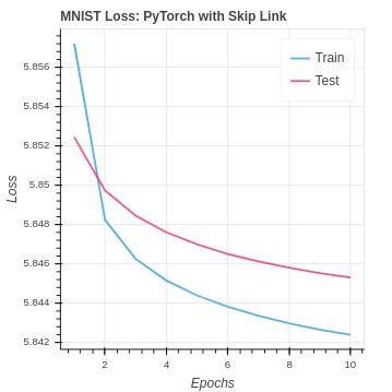
Here we implement an identity skip link to pass the pixel value input past the convolution layer. The values are then added together, and activation is applied. This strategy gives our fully connected layers direct access to the pixel inputs and the convolution outputs. In order to implement the skip link, we need update our ReLu class to take the original image and the pooling layer output. Then, those inputs are added together and activated with leaky ReLu. On the back-propagation pass, the incoming gradients are properly distributed. In regards to the MNIST dataset, our performance is similar to the original CNN and pooling implementations. We are still doing just as well, but the new information has not pushed us to the next level.

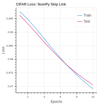
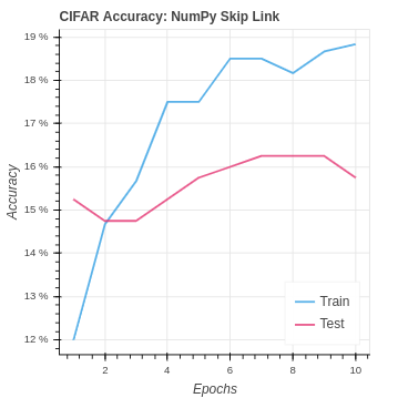
Extension 03 // Neural Network with Skip Link // Using NumPy

In the next section, we will see that the PyTorch implementation was able to do better. As a result, we can theorize that the less optimized naive NumPy may be responsible for the lack of gains. There are not stability guide rails built into the algorithms so our small gains are being lost. These studies give you a much greater appreciation of frameworks like PyTorch. Our NumPy CNN implementation was already struggling with the overwhelming amount of data in the CIFAR dataset and the more difficult class identification. With the added skip link data we are seeing a slight decrease in performance. It seems the network was already overwhelmed and does not have the capacity to extract a signal and learn from the additional data.

    class ReLu:
        # Use a fully connected layer using sigmoid activation

        def __init__(self, in_nodes, out_nodes):
            self.w = np.random.randn(out_nodes, in_nodes) / in_nodes
            self.b = np.zeros((out_nodes, 1))
            self.y_vector = np.zeros((1))
            self.z_cnn = np.zeros((1))
            self.a_cnn = np.zeros((1))
            self.z_out = np.zeros((1))
            self.a_out = np.zeros((1))
            self.image_size = 0


        def f(self, z):
            return np.where(z > 0, z, z * 0.2)

        def d_f(self, z):
            test = np.where(z>0, 1.0, 0.2)
            return np.where(z>0, 1.0, 0.2)

        def loss(self, y, yhat):
            self.y_vector = np.zeros((len(yhat), 1))
            self.y_vector[y, 0] = 1.0
            loss = np.linalg.norm(self.y_vector - yhat)
            accuracy = 1 if np.argmax(yhat[:, 0]) == y else 0
            return loss, accuracy

        def forward(self, image, x):
            # TODO setup to receive pool size
            h, w = image.shape
            self.image_size = h * w
            self.z_cnn = np.concatenate((image.reshape(-1, 1),  x.reshape(-1, 1)), axis=0)
            self.a_cnn = self.f(self.z_cnn)

            self.z_out = np.matmul(self.w, self.a_cnn) + self.b
            self.a_out = self.f(self.z_out)

            return self.a_out

        def back(self, alpha):

            w_grad = np.zeros(self.w.shape)
            b_grad = np.zeros(self.b.shape)

            # get delta for out layer
            delta_out = -(self.y_vector - self.a_out) * self.d_f(self.z_out)

            # get delta for hidden layer
            delta_pool = np.dot(self.w.T, delta_out) * self.d_f(self.z_cnn)

            w_grad += -alpha * np.matmul(delta_out, self.a_cnn.T)
            b_grad += -alpha * delta_out

            return delta_pool[self.image_size:]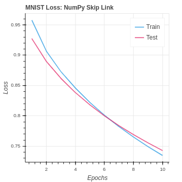

Extension 03 // Neural Network with Skip Link // Using PyTorch

In order to implement the skip link we will need to revise our Neural Network class.

class MNIST(nn.Module):

    # Our batch shape for input x is (1, 8, 8)

    def __init__(self):
        super(MNIST, self).__init__()

        # Input channels = 1, output channels = 18
        self.conv1 = torch.nn.Conv2d(1, 18, kernel_size=3, stride=1, padding=1)
        self.pool = torch.nn.MaxPool2d(kernel_size=2, stride=2, padding=0)
        self.fc1 = torch.nn.Linear(8 * 8 + 18 * 4 * 4, 64)
        self.fc2 = torch.nn.Linear(64, 10)

    def forward(self, x):
        in_x = x
        x = F.relu(self.pool(self.conv1(x)))
        in_x = in_x.view(-1, 8 * 8)
        x = x.view(-1, 18 * 4 * 4)
        x = torch.cat((in_x, x), 1)

        x = self.fc1(x)
        x = torch.relu(x)

        x = self.fc2(x)
        x = F.log_softmax(x, dim=1)

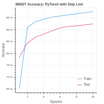
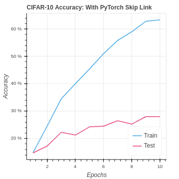
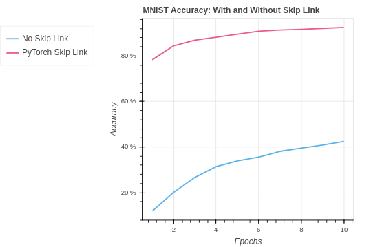
        return x

We see again how one size does not fit all in machine learning. Our PyTorch skip link model hits a new all-time best test set accuracy. The network was able to extract an improved signal and learn better using the extra data passed through the network to the fully connected layer.

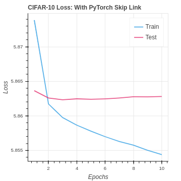
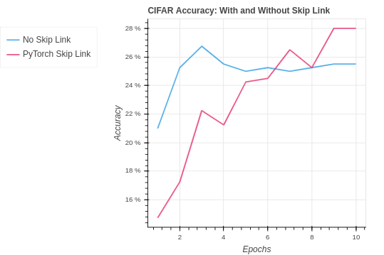
With the CIFAR-10 we see a similar performance to CNN with no skip link. It seems that the network is already at its max capacity to learn. To improve the performance on CIFAR-10 we will need to look into how to reduce over-fitting and increase the capacity. In the future, we could start to look into improvement by adding additional CNN layer blocks with skip links.

Extension 03 Synopsis

Algorithm	Training Set Accuracy	Test Set Accuracy
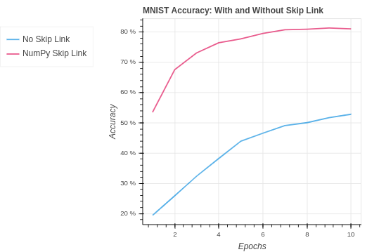
MNIST Baseline No Skip Link	29.50%	24.90%
MNIST NumPy Skip Link	86.83%	81.08%
MNIST PyTorch Skip Link	97.68%	92.49%
CIFAR Baseline No Skip Link	32.67%	25.25%
CIFAR NumPy Skip Link	18.83%	15.75%
CIFAR PyTorch Skip Link	63.33%	28.00%

Directories

Extension-1/

The directory containing the Baseline Neural Network without CNN and a Convolutional Neural Network extension. The extension is implemented in PyTorch and separately in NumPy. There are unique implementations of both for the two datasets MNIST and CIFAR-10. In addition, we explore the benefits that can be gained using Leaky ReLu over a Sigmoid activation.

Extension-2/

The directory contains a baseline neural network without extension. In addition, there are Convolutional Neural Networks that have been extended with Pooling layers. Pooling has been implemented using NumPy only and with PyTorch.

Extension-3/

The directory containing a baseline neural network without extension. In addition, there are convolutional neural networks that have been extended with the skip link strategy used by deep neural networks. Skip link has been implemented using NumPy only and with PyTorch.