A pytorch train demo with classical CNN models

First of all, in case of no dataset, we generate a dataset code in simplest way. The dataset consists of to parts, includeing the training value and the label. There training value represented by data and training label is represented by label

The code in Create_dataset.py is following

import numpy as np
# The number of samples simulated
numbers = 100
# The number of channel simulated
channels = 3
# The length of data simulated
length = 224
# The number of categories simulated
classes = 2

# Generate random data
data = np.random.randn(numbers,channels,length)
# Generate label
label = np.random.randint(0,classes,numbers)

# Saveing data and label to the Dataset file
np.save('Dataset/data.npy',data,allow_pickle=True)
np.save('Dataset/label.npy',label,allow_pickle=True)

np.random.randn demo

import numpy as np
data = np.random.randn(100,3,244)
print(data.shape)
# (100, 3, 244)

Using np.random.randint to generate label, The purpose of this code is to generate numbers of intergers contained in [0,classes)

label = np.random.randint(0,classes,numbers)

np.random.randint demo

import numpy as np

label = np.random.randint(0, 2, 10)
print(label)
# [0 0 0 1 1 0 1 0 0 0]

After runing this code, we generate two npy files under the Dataset folder

Before training out model, we need a function to packge the value and label that form is like [value，label],In order to split and train easily. This is a defoult form,if you are a new coders, you only need to just do it like this.

import numpy as np
def package_dataset(data, label):
    dataset = [[i, j] for i, j in zip(data, label)]
    # channel number
    channels = data[0].shape[0]
    # data length
    length = data[0].shape[1]
    # data classes
    classes = len(np.unique(label))
    return dataset, channels, length, classes


if __name__ == '__main__':
    data = np.load('Dataset/data.npy')
    label = np.load('Dataset/label.npy')
    dataset, channels, length, classes = package_dataset(data, label)
    print(channels, length, classes)
    #  3 224 2

This API input data and label , returndataset,channels,length,classes Follwing code is used to packge the data and label.

dataset = [[i, j] for i, j in zip(data, label)]

if it looks like a little abstract to a novice here's a simple example,By zip() and list generation a dataset consisting of multiple [value,label]is obtained

data = [[1, 2, 3],
        [3, 1, 3],
        [1, 2, 3]]

label = [0,1,0]

dataset = [[i, j] for i, j in zip(data, label)]

print(dataset)
#[[[1, 2, 3], 0], [[3, 1, 3], 1], [[1, 2, 3], 0]]

Now we will show the each part of the code step by step

import numpy as np
import torch
import matplotlib.pyplot as plt
from torch.utils.data import DataLoader, Dataset,random_split

Import our packge API

from Package_dataset import package_dataset

Import model, you can choose model which you need

from Models.LeNet import LeNet
from Models.AlexNet import AlexNet
from Models.ZFNet import ZFNet
from Models.VGG19 import VGG19
from Models.GoogLeNet import GoogLeNet
from Models.ResNet50 import ResNet50
from Models.DenseNet import DenseNet
from Models.SqueezeNet import SqueezeNet
from Models.Mnasnet import MnasNetA1
from Models.MobileNetV1 import MobileNetV1
from Models.MobileNetV2 import MobileNetV2
from Models.MobileNetV3 import MobileNetV3_large, MobileNetV3_small
from Models.shuffuleNetV1 import shuffuleNetV1_G3
from Models.shuffuleNetV2 import shuffuleNetV2
from Models.Xception import Xception
from Models.EfficientNet import EfficientNetB0

Loding dataset and read the value and label.

data = np.load('Dataset/data.npy')
label = np.load('Dataset/label.npy')

Number of how many times we train out model epoch_number

And train how many times to perform a test. show_result_epoch Why we need show_result_epoch, Due to sometime model trains to fast. If we print result after each epoch, Efficiency aside, you can't read the worlds when you keep print.

dataset_partition_rate = 0.7
epoch_number = 1000
show_result_epoch = 10 

Use our API package_dataset output dataset, channels, length, classes

dataset, channels, length, classes = package_dataset(data, label)

Split dataset, For this purpose , we use torch.utils.data.random_split, the random_split enter two parameters. One is dataset which is wating for split. There is also a list of lengths to pass on.

# partition dataset
train_len = int(len(dataset) * dataset_partition_rate)
test_len = int(len(dataset)) - train_len
train_dataset, test_dataset = random_split(dataset=dataset, lengths=[train_len, test_len])

Code the class of load dataset. This class is used to transform the raw dataset to a form which pytorch can understand. This allows the data to be used by tools such as Pytorch's Dataloader to train learning models.

class Dataset(Dataset):
    def __init__(self, data):
        self.len = len(data)
        self.x_data = torch.from_numpy(np.array(list(map(lambda x: x[0], data)), dtype=np.float32))
        self.y_data = torch.from_numpy(np.array(list(map(lambda x: x[-1], data)))).squeeze().long()

    def __getitem__(self, index):
        return self.x_data[index], self.y_data[index]

    def __len__(self):
        return self.len

Loading 'dataloder', 'train_dataset' and 'test_dataset' is' random_split 'to the input' dataset 'according to the ratio we set, divided the training set and the test set. In addition to the number of training samples contained by 'dataset', the data format of each training sample is the same as' [value, label] ' The official or most accurate expression of the phrase 'Train_dataset = Dataset(train_dataset)' is by instantiating the 'Dataset' to create a specific dataset object for the 'train_dataset' data preparation. Okay, I feel a little out of person, too. There is no need to tangle here to understand that we need to deal with the 'train_dataset' and 'test_dataset' separately through the 'Dataset', We then take the Train_dataset and the Test_dataset, respectively, and throw them into the DataLoader. The two variables' shuffle 'commonly used in' DataLoader 'to be set to' Ture 'is to scramble the input training set or test set, and then' batch_size 'refers to the size of the Mini-Batch strategy used in training.。

Train_dataset = Dataset(train_dataset)
Test_dataset = Dataset(test_dataset)
dataloader = DataLoader(Train_dataset, shuffle=True, batch_size=50)
testloader = DataLoader(Test_dataset, shuffle=True, batch_size=50)

Choose the training device, do you choose CPU training or GPU training, and what this code does is if cuda is available in general that means you're installing pytorch on a GPU then the default device is the GPU, and if you don't have a GPU, Then 'torch.cuda.is_available()' will return 'False' will select the CPU, generally speaking, we use our own laptop, or desktop when there is only one graphics card, if your device is a server, and installed multiple graphics cards in the case, Here 'cuda:0' can be set to other numbered 'cuda' such as' cuda:1 ' 'cuda:2' and so on

device = torch.device("cuda:0" if torch.cuda.is_available() else "cpu")

Before this time, we return 'channels',' length ', 'classes' in the' Package_dataset 'kind of function comes first, in the part of the model instantiation, will need to use this write parameter, if the adaptive pooling layer is used in the process of model construction, In general, there is no need to pass in the number of sample points, that is, the length of the value, so there are generally two cases, initialization needs to input the number of input channels, the number of categories, and the length of the value is also in the number of one-dimensional sample points, or only need to input the number of channels, and the number of categories. Where 'model.to(device)' is to deploy the model to the 'device' we selected in the previous step

# Initialize
# model = LeNet(in_channels=channels, input_sample_points=length, classes=classes)
# model = AlexNet(in_channels=channels, input_sample_points=length, classes=classes)
# model = AlexNet(in_channels=channels, input_sample_points=length, classes=classes)
# model = ZFNet(in_channels=channels, input_sample_points=length, classes=classes)
# model = VGG19(in_channels=channels, classes=classes)
# model = GoogLeNet(in_channels=channels, classes=classes)
# model =ResNet50(in_channels=channels, classes=classes)
# model =DenseNet(in_channels=channels, classes=classes)
# model =SqueezeNet(in_channels=channels, classes=classes)
# model =MobileNetV1(in_channels=channels, classes=classes)
# model =MobileNetV2(in_channels=channels, classes=classes)
# model =MobileNetV3_small(in_channels=channels, classes=classes)
# model =MobileNetV3_large(in_channels=channels, classes=classes)
# model =shuffuleNetV1_G3(in_channels=channels, classes=classes)
# model =shuffuleNetV2(in_channels=channels, classes=classes)
# model =Xception(in_channels=channels, classes=classes)
model =EfficientNetB0(in_channels=channels, classes=classes)
model.to(device)

For the selection of loss function, after instantiating the model, it is necessary to further select the degree of inconsistency between the results trained by the model and the actual results, that is, the size of the loss. The cross-error entropy loss function used in the following code, And this loss function can also be thought of as a model so you can move the loss function to the GPU in the same way that you move the model to the GPU. In the multi-classification task, the cross error entropy can be used directly for the loss function.

criterion = torch.nn.CrossEntropyLoss()
criterion.to(device)

Optimizer selection, because the core idea of deep learning algorithms is backpropagation and gradient descent, the role of the optimizer is to apply the loss to the parameter values that the original model can learn through the calculation of specified rules, of which there are two kinds worth using, one is' Adam 'and one is' SGD' plus momentum, and the others do not need to be tried.

# optimizer = torch.optim.Adam(model.parameters(), lr=0.001)
optimizer = torch.optim.SGD(model.parameters(), lr=0.001, momentum=0.9)

Initalize to list. they are used to save the accuracy of traindataset and test test.

train_acc_list = []
test_acc_list = []

Next is the most difficult part of the training function part, I will be very detailed to explain, the 'train' function for additional dismantling, if you are small white hope you do not be scared off, read this you will surpass the vast majority of people who can only copy and paste. First of all, 'train' function needs to pass a parameter is' epoch 'this parameter is the current number of rounds, the role of this parameter is to determine whether the current number of training rounds is an integer multiple of' show_result_epoch ', if it is to calculate the training set and accuracy of the accuracy of the test set.

def train(epoch):

Set the model to 'train' mode, and then execute the 'model.eval()' function when predicting the test set, two states mainly affect 'Dorpout' and 'BatchNormilze', take 'Dorpout' for example, if in 'train' mode, The nodes Droput drops each time he makes a prediction are random, but in 'eval' mode which node he drops is fixed. ** If you want to reproduce the results of the test set, you must add mode switching code during training and testing, otherwise the results will not be reproduced **

	model.train()

'train_correct' number of correct training set samples, 'train_total' is used to store the total number of all samples,

    train_correct = 0
    train_total = 0

'train_correct' number of correct training set samples, 'train_total' is used to store the total number of all samples

    for data in dataloader:
        train_data_value, train_data_label = data
        train_data_value, train_data_label = train_data_value.to(device), train_data_label.to(device)
        train_data_label_pred = model(train_data_value)
        loss = criterion(train_data_label_pred, train_data_label)
        optimizer.zero_grad()
        loss.backward()
        optimizer.step()

dataloader = DataLoader(Train_dataset, shuffle=True, batch_size=50)

Let's say the length of 'dataloder' is n, this dataloder is from this code, you can see that the size of 'batch_size' is set to 50, and let's say that the length of 'Train_dataset' we entered is 70, At last, the dataloder can get a sample of length 50 and a sample of length 20 through iteration. If the value of 'batch_size' is set to 10, then 7 samples of length 10 will be returned. If the value of 'batch_size' is set to 100, then a he of length 70 will be returned and he is not a v bully. So to sum it up, we're going to get three scenarios.

• When the value of batch_size is greater than the length of the first parameter 'Train_dataset' or 'Test_dataset' of the input 'DataLoader()', the iterator iterates over the data only once, The size of the data is the length of the input 'Train_dataset' or 'Test_dataset', that is, just to mess it up a bit, but the 'mini_batch' policy is not used
• When the value of 'batch_size' is less than the length of the first parameter 'Train_dataset' or 'Test_dataset' of the input 'DataLoader()', And the length of the input 'Train_dataset' or 'Test_dataset' is an integer multiple of 'batch_size' , Suppose the dataset length of input 'Dataloader' is n batch_size 'is b, and the number of iterations t=n|b. The | represents divisible, that is, the data length of each iteration can be iterated t times is b
• When the value of 'batch_size' is less than the length of the first parameter 'Train_dataset' or 'Test_dataset' of the input 'DataLoader()', And when the length of the input 'Train_dataset' or 'Test_dataset' is not an integer multiple of 'batch_size' , similarly assume that the dataset length of 'Dataloader' is $n$batch_size size is b, The number of iterations is t+1. The same t=n|b, the length of the data generated by the first iteration t is b, and the length of the last iteration is n-t×b

    for data in dataloader:

Do the following with the data from each iteration First of all, data contains two values, one is the value in this batch and the other is the label in this batch

        train_data_value, train_data_label = data

The resulting values and labels are then placed in 'device'

        train_data_value, train_data_label = train_data_value.to(device), train_data_label.to(device)

Then call the model to predict 'train_data_label_pred' as the predicted result, here it should be mentioned that the data dimension of this result is' (len(data),classes) ', 'len(data)' the data length of the local iteration to 'data'. 'classes' is the number of classes for the categorical task.

        train_data_label_pred = model(train_data_value)

Then call the model to predict 'train_data_label_pred' as the predicted result, here it should be mentioned that the data dimension of this result is' (len(data),classes) ', 'len(data)' the data length of the local iteration to 'data'. 'classes' is the number of classes for the categorical task.

        loss = criterion(train_data_label_pred, train_data_label)

Gradient clearing, calling the 'optimizer' 'zero_grad' method, will make clear the gradient saved for each learnable parameter, the reason for the need to separate this step is said to be reserved for the purpose of some tasks need to accumulate backpropagated gradients.

        optimizer.zero_grad()

Backpropagation gradient, which assigns a gradient to each learning parameter by backpropagation

        loss.backward()

Parameter update, using the gradient and the original parameters to get the parameters after this round of learning, the mode of action is to perform the following gradient descent, the specific mode of action depends on the selected optimizer.

        optimizer.step()

The following is the part of calculating accuracy and testing, 'epoch' is the current training round, 'show_result_epoch' is how many rounds to view the accuracy and loss of a training set and test set, and record the loss of the training set and test set to draw a change curve of accuracy.

    if epoch % show_result_epoch == 0:

By 'torch.max' to get the predicted label, 'torch.max' returns two values, one is the maximum probability 'probability', one is the index of the maximum 'predicted', which is what we think of as the label.

        probability, predicted = torch.max(train_data_label_pred.data, dim=1)

torch.max demo

import torch

data = torch.Tensor([[0.6, 0.4],
                     [0.3, 0.7]])


probability, predicted = torch.max(data.data, dim=1)

print(probability)
# tensor([0.6000, 0.7000])
print(predicted)
# tensor([0, 1])

Record the number of training samples to the variable 'train_total' that holds the total number of training samples, and the following 'size(0)' represents reading the first value of the Tensor dimension. For example, 'train_data_label_pred' dimension is' (20,2) '20 is the size of the' batch 'of this time, is the number of categories,' train_data_label_pred.size(0) 'is to take 20 out.

        train_total += train_data_label_pred.size(0)

Record the number of predicted samples that are correct. 'predicted == train_data_label' Compare the predicted label with the real label. This is a syntax. First the two Tensor have the same length, and then return an array containing 'true' and 'Flase'. The predicted labels of the corresponding positions are the same as "Ture" and the predicted labels are different as "False". Then add a ".sum() "in" (predicted == train_data_label) "to return the number of samples that are predicted correctly. A simple example is as follows: '.item() 'returns the value in Tensor.

        train_correct += (predicted == train_data_label).sum().item()

import torch

predicted = torch.Tensor([0, 1, 1, 0, 1])
train_data_label = torch.Tensor([0, 0, 1, 0, 1])

print(predicted == train_data_label)
# tensor([ True, False,  True,  True,  True])
print((predicted == train_data_label).sum())
# tensor(4)
print((predicted == train_data_label).sum().item())
# 4

Calculate the training set accuracy and add to 'train_acc_list', 'train_correct' is the number of correct predicted, 'train_total' is the total number of predicted samples, 'round' is used to scope floating-point numbers to how many decimal places.

        train_acc = round(100 * train_correct / train_total, 4)
        train_acc_list.append(train_acc)

print accuracy and loss

        print('=' * 10, epoch // 10, '=' * 10)
        print('loss:', loss.item())
        print(f'Train accuracy:{train_acc}%')

Complete traning section code

def train(epoch):
	model.train()
    train_correct = 0
    train_total = 0
    for data in dataloader:
        train_data_value, train_data_label = data
        train_data_value, train_data_label = train_data_value.to(device), train_data_label.to(device)
        train_data_label_pred = model(train_data_value)
        loss = criterion(train_data_label_pred, train_data_label)
        optimizer.zero_grad()
        loss.backward()
        optimizer.step()
    if epoch % show_result_epoch == 0:
        probability, predicted = torch.max(train_data_label_pred.data, dim=1)
        train_total += train_data_label_pred.size(0)
        train_correct += (predicted == train_data_label).sum().item()
        train_acc = round(100 * train_correct / train_total, 4)
        train_acc_list.append(train_acc)
        print('=' * 10, epoch // 10, '=' * 10)
        print('loss:', loss.item())
        print(f'Train accuracy:{train_acc}%')
        test()

Similarly, the test function is basically the same except that there is no backpropagation calculation loss and training process. The only thing that is more is that before entering the call iterator to read the test set sample, a 'with torch.no_grad()' is used to close the function related to gradient change. Here, when I just read it, I also wondered why I need to lock the following gradients every time I do backpropagation. The answer I got from learning is that even if the gradient is not used to update the parameter, if the gradient is not locked, PyTorch will track and store the intermediate value for automatic gradient calculation by default, which will affect the operation efficiency. It is also necessary to avoid gradient changes that may occur even if the gradient is not updated by the optimizer under certain circumstances, so the use of 'torch.no_grad()' is necessary.

def test():
	model.eval()
    test_correct = 0
    test_total = 0
    with torch.no_grad():
        for testdata in testloader:
            test_data_value, test_data_label = testdata
            test_data_value, test_data_label = test_data_value.to(device), test_data_label.to(device)
            test_data_label_pred = model(test_data_value)
            test_probability, test_predicted = torch.max(test_data_label_pred.data, dim=1)
            test_total += test_data_label_pred.size(0)
            test_correct += (test_predicted == test_data_label).sum().item()
    test_acc = round(100 * test_correct / test_total, 3)
    test_acc_list.append(test_acc)
    print(f'Test accuracy:{(test_acc)}%')

In order not to print the '0' training as a whole becomes' (1, epoch_number+1) ', this is not difficult but sometimes if you are confused or want to know why, you can change to range(epoch_number) and run to see.

for epoch in range(1, epoch_number+1):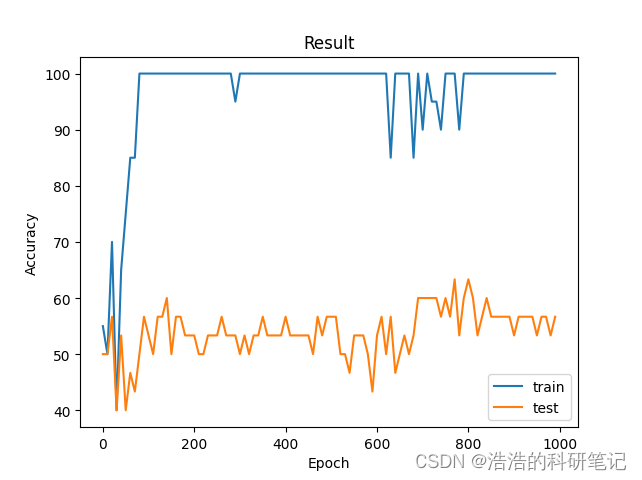
    train(epoch)

plt.plot(np.array(range(epoch_number//show_result_epoch)) * show_result_epoch, train_acc_list)
plt.plot(np.array(range(epoch_number//show_result_epoch)) * show_result_epoch, test_acc_list)
plt.legend(['train', 'test'])
plt.title('Result')
plt.xlabel('Epoch')
plt.ylabel('Accuracy')
plt.show()

The number of training rounds is 1000, and the final results are as follows, ** Since our data is a randomly generated binary classification dataset, the accuracy of the test set eventually moves up and down by 50%. **.

I hope you can look at the above content before looking at the complete code below, and then you will no longer be afraid of the following code will have a transparent feeling.

import numpy as np
import torch
import matplotlib.pyplot as plt
from torch.utils.data import DataLoader, Dataset,random_split
from Package_dataset import package_dataset

from Models.LeNet import LeNet
from Models.AlexNet import AlexNet
from Models.ZFNet import ZFNet
from Models.VGG19 import VGG19
from Models.GoogLeNet import GoogLeNet
from Models.ResNet50 import ResNet50
from Models.DenseNet import DenseNet
from Models.SqueezeNet import SqueezeNet
from Models.Mnasnet import MnasNetA1
from Models.MobileNetV1 import MobileNetV1
from Models.MobileNetV2 import MobileNetV2
from Models.MobileNetV3 import MobileNetV3_large, MobileNetV3_small
from Models.shuffuleNetV1 import shuffuleNetV1_G3
from Models.shuffuleNetV2 import shuffuleNetV2
from Models.Xception import Xception

data = np.load('Dataset/data.npy')
label = np.load('Dataset/label.npy')

dataset_partition_rate = 0.7
epoch_number = 1000
show_result_epoch = 10

dataset, channels, length, classes = package_dataset(data, label)

# partition dataset
train_len = int(len(dataset) * dataset_partition_rate)
test_len = int(len(dataset)) - train_len
train_dataset, test_dataset = random_split(dataset=dataset, lengths=[train_len, test_len])


# 数据库加载
class Dataset(Dataset):
    def __init__(self, data):
        self.len = len(data)
        self.x_data = torch.from_numpy(np.array(list(map(lambda x: x[0], data)), dtype=np.float32))
        self.y_data = torch.from_numpy(np.array(list(map(lambda x: x[-1], data)))).squeeze().long()

    def __getitem__(self, index):
        return self.x_data[index], self.y_data[index]

    def __len__(self):
        return self.len


# 数据库dataloader
Train_dataset = Dataset(train_dataset)
Test_dataset = Dataset(test_dataset)
dataloader = DataLoader(Train_dataset, shuffle=True, batch_size=50)
testloader = DataLoader(Test_dataset, shuffle=True, batch_size=50)
# 训练设备选择GPU还是CPU
device = torch.device("cuda:0" if torch.cuda.is_available() else "cpu")

# 模型初始化
# model = LeNet(in_channels=channels, input_sample_points=length, classes=classes)
# model = AlexNet(in_channels=channels, input_sample_points=length, classes=classes)
# model = AlexNet(in_channels=channels, input_sample_points=length, classes=classes)
# model = ZFNet(in_channels=channels, input_sample_points=length, classes=classes)
# model = VGG19(in_channels=channels, classes=classes)
# model = GoogLeNet(in_channels=channels, classes=classes)
# model =ResNet50(in_channels=channels, classes=classes)
# model =DenseNet(in_channels=channels, classes=classes)
# model =SqueezeNet(in_channels=channels, classes=classes)
# model =MobileNetV1(in_channels=channels, classes=classes)
# model =MobileNetV2(in_channels=channels, classes=classes)
# model =MobileNetV3_small(in_channels=channels, classes=classes)
# model =MobileNetV3_large(in_channels=channels, classes=classes)
# model =shuffuleNetV1_G3(in_channels=channels, classes=classes)
model =shuffuleNetV2(in_channels=channels, classes=classes)
# model =Xception(in_channels=channels, classes=classes)
model.to(device)

# 损失函数选择
criterion = torch.nn.CrossEntropyLoss()
criterion.to(device)
# 优化器选择
# optimizer = torch.optim.Adam(model.parameters(), lr=0.001)
optimizer = torch.optim.SGD(model.parameters(), lr=0.001, momentum=0.9)

train_acc_list = []
test_acc_list = []


# 训练函数
def train(epoch):
	model.train()
    train_correct = 0
    train_total = 0
    for data in dataloader:
        train_data_value, train_data_label = data
        train_data_value, train_data_label = train_data_value.to(device), train_data_label.to(device)
        train_data_label_pred = model(train_data_value)
        loss = criterion(train_data_label_pred, train_data_label)
        optimizer.zero_grad()
        loss.backward()
        optimizer.step()
    if epoch % show_result_epoch == 0:
        probability, predicted = torch.max(train_data_label_pred.data, dim=1)
        train_total += train_data_label_pred.size(0)
        train_correct += (predicted == train_data_label).sum().item()
        train_acc = round(100 * train_correct / train_total, 4)
        train_acc_list.append(train_acc)
        print('=' * 10, epoch // 10, '=' * 10)
        print('loss:', loss.item())
        print(f'Train accuracy:{train_acc}%')
        test()


# 测试函数
def test():
	model.eval()
    test_correct = 0
    test_total = 0
    with torch.no_grad():
        for testdata in testloader:
            test_data_value, test_data_label = testdata
            test_data_value, test_data_label = test_data_value.to(device), test_data_label.to(device)
            test_data_label_pred = model(test_data_value)
            test_probability, test_predicted = torch.max(test_data_label_pred.data, dim=1)
            test_total += test_data_label_pred.size(0)
            test_correct += (test_predicted == test_data_label).sum().item()
    test_acc = round(100 * test_correct / test_total, 3)
    test_acc_list.append(test_acc)
    print(f'Test accuracy:{(test_acc)}%')


for epoch in range(1, epoch_number+1):
    train(epoch)

plt.plot(np.array(range(epoch_number//show_result_epoch)) * show_result_epoch, train_acc_list)
plt.plot(np.array(range(epoch_number//show_result_epoch)) * show_result_epoch, test_acc_list)
plt.legend(['train', 'test'])
plt.title('Result')
plt.xlabel('Epoch')
plt.ylabel('Accuracy')
plt.show()

• Optimizer only Adam and SGD plus momentum is worth trying SGD momentum is generally set to 0.9
• The fastest way to improve accuracy is to normalize the data during data preprocessing, followed by BatchNormalize after the convolution layer
• Change the ReLu function to LeakLyRelu when there is no change in accuracy, i.e., the gradient disappears
• For one-dimensional data, ResNet tends to have the highest accuracy in the base model
• Piling attention mechanisms and recurrent neural networks on top of the model has a high probability of improving accuracy and is not recommended if you are trying to do something good
• The cuda memory error is that the batch_size is set too large, or the memory usage is too much, and the restart cannot be changed to a smaller batch_size
• bat_size hyperparameters such as the number of convolution layers are set to an integer multiple of the number of cores being processed, usually a multiple of 32