Effect existence indices in the Bayesian framework paper/vignette about easystats HOT 315 CLOSED

I updated the new data, and recompiled the vignette... but the size of the package went up (above CRAN's limit) due to the images and all no matter how I tried, so in the end I moved the draft here for now.

Also, after re-reading it all, I think it would be better to stick with "study 1" (where we modulate the sample size and the noise), there will already quite a lot of things to discuss.

Once this paper it out, we might summarise it in the vignette and redirect to the full paper ☺️

from easystats.

It was more a general comment on overhyping, not specifically addressing you ;-)
But I think this is in general not uncommon that when you switch from frq to Bayes, you see all the benefits, and you start seeing only benefits (at least this was what I observed for me personally).

from easystats.

definitely... Sander's comments are quite refreshing, it's rare to read well-informed and provoking takes on frequentist indices

from easystats.

Okay, I'll have a look once we have the new data. Let's add this in a list so we don't forget:

• add marginal densities to p-value comparison

from easystats.

https://journals.plos.org/ploscompbiol/article?id=10.1371/journal.pcbi.1007128
https://manubot.org/

👀

from easystats.

Can you guys fork the other repo and push there?

from easystats.

The journal requires AE.

from easystats.

I've restarted the generation with the updated bayestestR (the rope's range) with only 50 iter of noise level instead of 1000, so the data should be ready this evening. This way we can check if everything is reasonable this time and start working with this preliminary data on things like plots and all while the full generation is running.

from easystats.

In the end I came up with a kind of "flexible" rope-rage, depending on the probability of success (something like Kruschke suggests, but only tests for the 50:50 case). My "formula" is here. But Dominique wasn't convinced, and it was still a bit mystic to us, so we used a fixed range ;-)

from easystats.

@strengejacke I still cannot wrap my head around selecting ROPE ranges (I use to think the ROPE was just the ~[half minimal change in Y of interest], so the reason why we defining a range for X, or why we divide by 4 is beyond me 🤷‍♀️ )... I really should get back to Kruschke's book...

from easystats.

Kruschke's reasoning is based on an "effect size", as defined by Cohen. Cohen's D is the standardized mean difference, i.e. a difference of x SD. A small effect is D ~ 0.1. So for linear models, the ROPE is 0.1 * SD(y). This does not work for logistic regression models (we have no real standard deviation for a binary outcome). I think, the "4-stuff" maybe comes from the Division by 4 rule - but maybe he just likes that number...

from easystats.

I think we'll leave that for last - after we get all the bit and pieces we want in the plot, I'll work my maggic (maggic=ggplot+magic) 😊

from easystats.

We'll hopefully see more clearly when the full data set will be available :)

from easystats.

Hey, that's their problem 😜
Here are two reasons to include both in the paper:

1. 100% prior that a reviewer will say "but BFs are sensitive to prior specification!". This would somewhat deal with that.
2. I'd sleep better at night?

from easystats.

That sounds good! I'm always open to and happy about writing a paper on Bayesian analysis, because I would like to have some "citeable" references. :-)

I think, though, that such a paper would benefit from a wording that does not overhype the Bayesian philosophy. There's a very interesting discussion here:
https://discourse.datamethods.org/t/language-for-communicating-frequentist-results-about-treatment-effects/934/16

and an important comment later on here:
https://discourse.datamethods.org/t/language-for-communicating-frequentist-results-about-treatment-effects/934/28

Frequentist results are chronically misrepresented and hence miscommunicated. Yes their Bayesian counterparts can be phrased more straightforwardly, but that’s not always an advantage because their overconfident descriptions are harder to see as misleading. “The posterior probability” is a prime example because there is no single posterior probability, there is only a posterior probability computed from a possibly very wrong hierarchical (prior+data) model. Similarly there is no single P-value for a model or hypothesis.

from easystats.

Though this is "just" another opinion from Sander, I find it convincing and see the point that just using Bayesian methods does not overcome all existing problems.

from easystats.

this is very interesting, I am indeed guilty of overhyping it 😅

from easystats.

I think that decomposing the paper/vignette in 3 could be clearer than modulating and assessing the effect of everything at once.

I was thinking about 3 "experiments" (or parts):

• one in which are modulated effect size, sample size and noise, in which we compare the indices and their relationship with frequentist ones. For this part, the generation script is pretty much in shape. I need to update the data for the vignettes by re-running it again(it's in circus, I'd be glad to have your input), which takes about a week on a server 😞. I will start it right after I finish with my current scripts for a paper revision (which is due next week).
• a second experiment to investigate the sensitivity of indices to priors specification. I am not sure yet of the best way to investigate that. I was thinking of generating data with 3 different types of priors, located at 0, at the "true" effect (although defining this is a bit of a pickle) and at the inverse of the true effect. And see how it affects the indices.
• a third experiment could test the robustness to sampling quality. One way to test that could be modulating the sampling characteristics such as the number of chains, burn-in, draws, algorithm etc.

from easystats.

I finally am done with a personal analysis. So I am planning to re-run the script to obtain the data for the indices of effect existence vignette (which will take about 1 week).

I am planning to add 2 indices for each coef's posterior:

• BF - savage dickey with prior rcauchy_perfect with location 0 and scale = SD of the posterior
• BF - savage dickey with prior rcauchy_perfect with location 0 and scale = 1

Mainly out of curiosity, to see how it relates to other indices such as ROPE and so on.

here is the code used to extract the relevant indices. Let me know if you have any suggestions about other indices.

from easystats.

@DominiqueMakowski I am also interested to see how these heuristic priors work out in the new BF-SD. Please keep me posted!

from easystats.

@DominiqueMakowski As stanreg models are now supported by the Savage-Dickey BF function, which extracts actual priors directly, maybe you could add that to the vignette as well!

(I feel very at home here, as you can tell by how comfortably I allow myself to suggest some extra work for you 😄 )

from easystats.

Yes, I think I'll replace the current two BFs (Cauchy 0.707 and Cauchy 1) by Cauchy 0.707 and model's priors.

from easystats.

I was looking at the Comparison of Indices of Effect Existence, and had some thoughts regarding the BFs:

1. Am I correct to assume that the prior scales are standardized?
2. I think it would be interesting to have 2*2 bayes factors:
   1. Model comparison BF (effect model vs intercept only model) and Savage-Dickey (posterior vs prior).
   2. Prior ~cauchy(0, 0.707) / ~student_t(3, 0) (autoscaled) - these seem to be the two most popular options.
3. I find it very weird that when the null is true, the log(BF) never goes bellow -2.5, even as sample size increases and noise is low, which is inconsistent with other works. On that note...
4. Unless I am reading the vignette wrong (which is totally possible), none (or at least most?) of the indices seem to be informative when the null is true (all seem to behave similar to the p-value) which is disapointing, as the main draw to Bayesian stats is often the ability to support the null. Does only the ROPE+equi allow for this?

from easystats.

For the BF part:

• this vignette takes focus in the characteristics on the parameters only, not the entire model (thus model comparison BFs would be for another vignette :)
• due to our recent changes and direct support of sdBF for rstanarm, I'd say it's best if we keep only this BF the way it is computed by bayestestR

For other weirdnesses in the data, it needs to be re-generated anyway, so I would mainly focus on making sure the generating script is ok (as it takes a long time to run, so we have to make sure it works as expected :).

from easystats.

@strengejacke @mattansb
I have reformatted the code related to the simulation study: see here.

Please try to have a look if you find the time (I know it's not a page-turner), I would like to have your opinion before running the simulation on the server.

While I think that study 1 (comparison with frequentist models and effect of sample size and error) and study 2 (effect of sampling characteristics) are "working" (although let me know if the boundaries for the parameters tested make sense for you), I have a problem with study 3; which aims at investigating the effect of prior specification.

In my opinion, I think it would be interesting to compare 3 types of priors, the default (uninformative, centred around 0) with a congruent prior (in the sense of the effect) and an incongruent (in the opposite of the effect's direction). For the linear models, this is not a problem. The true effect is either 0 or 1 (roughly corresponding to a perfect correlation). Thus, in the case a true effect is 1, a congruent prior is normal(1, 1) and an incongruent prior is normal(-1, 1).
But things get more complicated in the case of logistic models, as the actual coefficient of a "perfect" correlation is quasi-undefined (but it is clearly higher than 1):

In this context, how to specify an "informative" prior so that it is comparable (in terms of magnitude) between linear and logistic models? Any ideas?

from easystats.

Some notes / questions:

1. I think that the params$BF_cauchy07 part is kind of cheating - you're not really specifying the prior on which the posterior is based here, you're just "feeding" sdBF a distribution to compare against, which might give bogus results:

params$BF_cauchy07 <- as.numeric(bayesfactor_savagedickey(posterior,
                                    prior = distribution_cauchy(length(posterior),
                                                                location=0,
                                                                scale=0.707),
                                    hypothesis = 0,
                                    verbose=FALSE))

2. The code for the actual sdBF can be simplified (shouldn't add much processing time considering such small Ns / simple models) to:

params$BF <- bayesfactor_savagedickey(models$bayesian)$BF[2]

3. Unless I'm reading the code wrong - is the max noise set at 0.66? If so, this corresponds to r = 0.8, which is quite large. I would go to maybe max error/noise of 5 (for r = 0.15) maybe even more?

Other than that, code seems alright :)

from easystats.

@mattansb

1. You're right, I'll remove this BF to only use the one using the model's priors.
2. I would have thought so too :) Unfortunately, it doesn't work if I pass the model directly... Nore sure why, but my guess is that it can't retrieve the model properly as the model is passed too deeply and is not accessible from the global scope 😕
3. The noise is actually from 0.33 to 6.66, I am not sure where you got the 0.66 value 🤔

from easystats.

3. The noise is actually from 0.33 to 6.66, I am not sure where you got the 0.66 value 🤔

Oops, I seem to have seen that first 6 as a 0...

from easystats.

When would you like to have feedback on this?

from easystats.

whenever you can, no pressure, it is not urgent
(though needed to generate the data for the vignettes/paper) ;)

from easystats.

A minor change, in plotting: I it would be good to add marginal density plots / histograms to the plots comparing all the measures to frequentist p-values. This will show that the Bayesian measures are consistent when H0 is true (i.e., they converge), which is not the case for the p-values (that converge when H1 is true, but have a uniform distribution when H0 is true).

from easystats.

Good point! If you know how to nicely add the marginal densities, could you add them to the vignette?

from easystats.

I do not... I this this can be done with ggExtra, though I've never used it before... and I don't know how it deals with faceting...

from easystats.

How do we compile the RMD to have a "readable" version for the paper, and how should we edit?

from easystats.

I have knitted a readable version in word (using frontiers template) but indeed we can reknit it in a md or pdf format it will be easier to check

from easystats.

Alright - how to you wish to proceed?

(Or: how can I comment? 😅)

For now I'm writing my comments here, so I don't forget them:

1. Figure 4 (Relationship with frequentist p-based arbitrary clusters) - I would make two changes:

   1. Split the figure in to two: one where there is an effect and another where there isn't - this would give some mapping for the indices onto power / false discovery.
   2. Combine all the alpha thresholds into one plot with multiple s-curves:
      

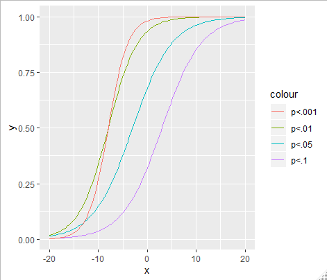
2. I think the "noise" parameter should be followed with the equivalent "effect size", which I think people are more use to thinking about.

from easystats.

If not, it might be easier to createand make more sense to create a devoted repo for that, for instance under easystats/easystats/publications or something along those lines, where we would store papers and data related to the project?

from easystats.

under easystats/easystats/publications

I think would be easier for collab

from easystats.

I agree, I'll transfer

from easystats.

moved

from easystats.

Could you please elaborate a bit on the figures in the paper? They're still confusing to me... E.g.:

3.1.2 Sensitivity to Sample Size

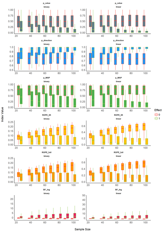
Does it mean that for no effect, the p-value was mostly not associated with sample size, and for a true effect, p-values were lower with increasing sample size?

And how to interprete the ROPE panels?

from easystats.

from easystats.

I think we have quite some work to do with the paper.

• Sections Methods and Results are missing (for results, at least the text)
• Discussion needs more content
• Introduction is far too long and not focussing on our topic, so it also needs some major revisions, to make it clear to the reader what we want (we should move the presentation of the indices to the methods section, this will already shorten the introduction)
• The figures probably need to be presented differently. I would suggest using two colors (true effect/no effect), and no outline. Currently we have a new color for each panel, and it's not clear why. I think it will be sufficient to have titles for the panels, and not additionally new colors, because this will distract from the fact that we compare true to no effects
• Furthermore, we mix figures for Freq and Bayes models, we should explain the reasoning behind this. And we need to make clearer why we both have Freq and Bayes models in our simulation.
• In the methods section, we must justify the indices we present (and this should typically be derived from the introduction, to have a "logical" structure that is easy to follow).

I can make a first step, but I would like to clarify #33 (comment) first.

What do you say?

from easystats.

I agree on all points. I can get working on the plots (as I've already made changes to figure 4).

I feel like I'm kind of hovering around this paper right now, so if there is anything you fell / want / think I should be more involved with, please let me know.

from easystats.

I feel like I'm kind of hovering around this paper right now

It's me that is definitely hovering around it currently ^^ (as you can see through how I ignored all comments pertaining to it haha), I'll try answering the comments this evening/tmr, but I can predict that I agree with all of them! All the plots need to be redone or at least substantially improved, as pretty much everything else

from easystats.

I've re-done figures 1-4 (I'm not quite sure what we're trying to show in figs 5-6, so didn't touch these for now). Instead of reknitting the paper, I saved the figures at .pngs (except for Figure 3, which is too complex for my tiny computer to render... If one of you could render this figure and save it, would love to see it 😅).

Some thoughts from looking at figures 1 & 2:

• It seems very weird that the BFs show only very limited support for H0 in any of the simulations... I know that it's over all harder to support H0 (since it's harder to distinguish small effects from no effects without very large Ns...), but still - disappointing 🤔
  • In fact, of all indices, ROPE seems to be the only one that shows more true support for H0 as sample size increases (when H0 is true) - thought from the works of Wagenmakers, Rouder, Morey et al, this should also be true for BF. Maybe because max N is 100? I don't know...
  • Also, any idea why the BF plots have so much empty space?
• For linear models, when H0 is true, ROPE in on average at 50%. But for binary it's on average 10% - are we sure the ROPE range for logistic models is properly defined? (This is the only index to show such a difference between the two model types).

from easystats.

It seems very weird that the BFs show only very limited support for H0 in any of the simulations... I know that it's over all harder to support H0 (since it's harder to distinguish small effects from no effects without very large Ns...), but still - disappointing

Recent tweet by Wagenmakers seems to suggest the this 👆 finding is not surprising - evidence is accumulated faster for the alternative (when it is true) than for the point-null (when it is true). Paper by Valen Johnson seems (? Didn't fully read or understand) that using an interval-null (instead of a point) makes this problem less severe - that is, when the null is true, evidence is accumulated in its favor faster. The simulation in the interval-null BF paper by Morey and Rouder (figure 5) also demonstrates this. (Both papers can be used for our discussion..).

Here is a little simulation I did to confirm (very quick and dirty, so not super accurate, but gets the point across; basically recreating fig 5 from Morey and Rouder):

As you can see, when H0 is true (red), for interval BF (solid line), the evidence accumulation is faster compared to point null (dotted line).

_{If it's not too late (which I suspect it is) I would suggest adding an interval-null BF to the simulation...}

from easystats.

TO DISCUSS / TO DO

1. add marginal densities to p-value comparison

2. Figure 4 (Relationship with frequentist p-based arbitrary clusters) - I would make two changes:
   Split the figure in to two: one where there is an effect and another where there isn't - this would give some mapping for the indices onto power / false discovery.
   Combine all the alpha thresholds into one plot with multiple s-curves:

3. If it's not too late (which I suspect it is) I would suggest adding an interval-null BF to the simulation...

Can, but it's gonna take a week (but it should not cause any breaks so we can still work on the rest). Can you add the line here. BF_interval is a good name for the index 😉

4. Could you please elaborate a bit on the figures in the paper?

5. Sections Methods and Results are missing (for results, at least the text)

6. Discussion needs more content

7. Introduction is far too long and not focussing on our topic, so it also needs some major revisions, to make it clear to the reader what we want (we should move the presentation of the indices to the methods section, this will already shorten the introduction)

I agree that the presentation of indices should be moved to methods. However, I would not remove too much of the "intro do Bayesian stats" paragraphs, as the audience and the readers of this paper might consist of a good proportion of non-experts (as it creates some parallel with the frequentist framework and attempts at drawing guidelines for reporting, which both are of particular interest to new Bayesianists)

8. The figures probably need to be presented differently. I would suggest using two colors (true effect/no effect), and no outline. Currently we have a new color for each panel, and it's not clear why. I think it will be sufficient to have titles for the panels, and not additionally new colors, because this will distract from the fact that we compare true to no effects

9. Furthermore, we mix figures for Freq and Bayes models, we should explain the reasoning behind this. And we need to make clearer why we both have Freq and Bayes models in our simulation.

10. In the methods section, we must justify the indices we present (and this should typically be derived from the introduction, to have a "logical" structure that is easy to follow).

11. 've re-done figures 1-4

from easystats.

Can we agree on using British spelling 😬?

from easystats.

.1. I added geom_rug to the plot (but was unable to render to see what it looks like). If this doesn't work, I'll add the marginal densities

.2. Changed my mind ^_^ see the new figure as it is now.

.3. Done (I've also changed the regular BF code a bit).

.8. I've mostly addressed this in point 11.

Can we agree on using British spelling 😬?

I'll try my best...........

from easystats.

I restarted the generation script :)

from easystats.

Mmh there is something wrong, while with the older code for regular BF it takes about 8 sec/iteration, with the new one for point-null BF it takes like forever... Could you check what's wrong? Maybe it has to do with the internal .update_to_priors?

from easystats.

Can we agree on using British spelling

The journal requires AE.

from easystats.

The journal requires AE.

😠

from easystats.

@DominiqueMakowski Had a little bug there - ran the first iteration to test that everything works, took about 6 seconds on my PC. Let me know if this is still an issue...

from easystats.

@mattansb the patch seems to work 🎉

from easystats.

For linear models, when H0 is true, ROPE in on average at 50%. But for binary it's on average 10% - are we sure the ROPE range for logistic models is properly defined? (This is the only index to show such a difference between the two model types).

@DominiqueMakowski @strengejacke (ROPE experts!) Do you think this is an artifact of the code specs (if so, prob wise to stop the sim for now)? Or does this seem like a reasonable finding to you?

from easystats.

Just realised that we might have done a mistake there 😱:

We had a long discussion about rope default selection for logistic models. In the end, the rope definition for a standardized parameter of a logistic model was (and is currently) derived from Cohen's conversion between standardized differences (Cohen's d) and log odds. The -0.055; 0.055 comes from d * sqrt(3)/pi = 0.1 * sqrt(3)/pi. Based on that, I did simply think that the equivalence was not perfect as shown by our data (the ROPE indices were not perfectly matching between models).

But now I just run parameters::d_to_odds(0.1, log = TRUE) which gave 0.1813799... So something was off. I looked at the formula again, and in fact, we might have inversed the terms: it should be 0.1 * sqrt(3)/pi... 😱 do you read the same thing as me?

from easystats.

You mean you did 0.1 * sqrt(3) / pi, when you should have done 0.1 * pi / sqrt(3)...?

Good thing we caught this just in time for a bayestestR release (:

from easystats.

You mean you did 0.1 * sqrt(3) / pi, when you should have done 0.1 * pi / sqrt(3)...?

in my defense I was confused by Daniel's obscure formulae, and critically we didn't have a Mattan to show us the light

from easystats.

Haha I only meant to make sure I understood you correctly!

Funny thing is, when I was just last week writing this blogpost I kept making the exact same pi / sqrt(3) vs sqrt(3) / pi mistake!

from easystats.

I think we ended up trying to decipher what Kruschke was saying, see here.

Here's a screenshot from the supplemental file:

Assuming (which is not always true) a 50/50 division from the binary outcome, a ROPE for logistic regression model often ends up being -.05 to .05 for negligible standardized regression coefficient.

from easystats.

I cleaned up a bit and made some touches to the figures related to the new (preliminary) data (which seems to work - so I'll restart the full gen), but I must say you guys greatly improved them. Tell me what you think now (I've set the Rmd to automatically save them in the figures folder)!

Intro

• Refactor and streamline intro

Methods

• Details and refs for BF interval

Results

• Figures legends need to be completed
• Result section needs more text

Discussion

• Write discussion

from easystats.

Something is wonky with the table in the PerformanceComparison chunk - some indices are out of order... right now looking at BF. This is the results of performance::compare_performance:

performance::compare_performance(p_value, p_direction, p_MAP, ROPE_95, ROPE_full, BF_log, BF_ROPE_log)
#>         Model Type      AIC       BIC   R2_Tjur      RMSE   LOGLOSS SCORE_LOG SCORE_SPHERICAL       PCP           BF
#> 6     ROPE_95  glm 917.4399  936.6495 0.3343392 1.0052307 0.5052444      -Inf     0.001383628 0.6671696 1.200575e+28
#> 7   ROPE_full  glm 914.3902  933.5998 0.3364456 1.0035439 0.5035501      -Inf     0.001410443 0.6682228 1.696956e+28
#> 2 BF_ROPE_log  glm 869.2629  888.4725 0.3590019 0.9782427 0.4784794      -Inf     0.001529036 0.6795010 8.542274e-01
#> 3 p_direction  glm 999.5805 1018.7900 0.2651042 1.0496457 0.5508780      -Inf     0.001772762 0.6325521 6.352962e+14
#> 1      BF_log  glm 869.9550  889.1645 0.3574368 0.9786357 0.4788639      -Inf     0.001679734 0.6787184 1.000000e+00
#> 4       p_MAP  glm 931.0951  950.3047 0.3254020 1.0127493 0.5128306      -Inf     0.001693825 0.6627010 5.863713e+17
#> 5     p_value  glm 999.2653 1018.4749 0.2654434 1.0494789 0.5507030      -Inf     0.001426051 0.6327217           NA

Now look at the same BF from the original bayestestR::bayesfactor_models:

bayestestR::bayesfactor_models(p_value, p_direction, p_MAP, ROPE_95, ROPE_full, BF_log, BF_ROPE_log)
#> # Bayes Factors for Model Comparison
#> 
#>   Model                                 Bayes Factor
#>   [2] p_direction + error + sample_size         0.85
#>   [3] p_MAP + error + sample_size           6.35e+14
#>   [4] ROPE_95 + error + sample_size         5.86e+17
#>   [5] ROPE_full + error + sample_size       2.69e+18
#>   [6] BF_log + error + sample_size          1.20e+28
#>   [7] BF_ROPE_log + error + sample_size     1.70e+28
#> 
#> * Against Denominator: [1] p_value + error + sample_size
#> *   Bayes Factor Type: BIC approximation

One value is missing (replaced by NA) and they're all out of order.

from easystats.

(I think some plots will have to be slip up for scaling (e.g, we'd want both ROPEs and both BFs to be on the same y scale) and then stiched together with cowplot or something.)

from easystats.

(I think some plots will have to be slip up for scaling (e.g, we'd want both ROPEs and both BFs to be on the same y scale) and then stiched together with cowplot or something.)

In which plots?

Something is wonky with the table in the PerformanceComparison chunk

Is it aused by compare_performance?

from easystats.

Something is wonky with the table in the PerformanceComparison chunk

Although when I run it seems okay... have you updated everything lol?

from easystats.

have you updated everything lol?

After updating everything works 😅 sorry...

In which plots?

I think in figure 1, 2, 3 & 5 we need to scale the y axis, and in figure 4 we need to scale the x axis, so they are the same for both ROPES and the same for both BFs (for the BFs I would also change the labels to represent the common thresholds, as I did here>>). The figures will generally look the same, this will just give a better basis for visual comparison between similar indices.

from easystats.

Right, it would be nice to have that y axis as in your figure... but I don't see how to do it since the current figure is facet_grid, and I am not sure if it's possible to change like individual scales in the panels... And doing it separately and assembling them later on might in turn ruin the current unified field (where there is only one x and y axis title) 🤔 🤔 Feel free to try to improve it tho ☺️

from easystats.

I am also not sure about what text to add to the results... describe the figures? Force in the report of some statistics?

from easystats.

I've added some comments (all marked inside HTML comments with MSB:).

Thought - do we want to add a section regarding the arbitrary thresholds of the pd (>97%~) ROPE (>99%, <1%), and BF (>3, <1/3)? (To talk about the calibration of these threshold?) Or is that beyond the scope of this paper?

from easystats.

I am also not sure about what text to add to the results... describe the figures? Force in the report of some statistics?

I think the style now, of mostly describing the figures, if good - the figures are very "rich", and it is necessary to guide the reader through them. I also really like the sensitivity table ^_^

from easystats.

do we want to add a section regarding the arbitrary thresholds

I think we could add a section "Reporting guidelines" with template sentences + interpretation heuristics, after all this paper aims to be rather of practical usefulness than theoretical considerations.

I also really like the sensitivity table ^_^

I wonder why 😅

from easystats.

I meant more in the lines of "are these threshold calibrated", but that might be too much to take on. I'll try and add a visual signifier in the plots, for readers convenience.

I wonder why 😅

I was honestly surprised! I've slowly been growing apart from BFs (we're in couples counselling 😜) due to the sensitivity to priors - I was slowly being converted to ROPE tests, but these results are quite strong! (I love that we compared Bayesian indices with BFs)

from easystats.

Figure 2: Noise is proportional to 1/(standardized effect size), so:
Does is make sense to even show the "effect = 0" in figure 2?

• Maybe add it on the far right at "Noise = Inf"?
• Or relabel the x axis as "standardized effect size" (and add all of "effect = 0" on the far left)?

Maybe re-struct results:

1. Sample size + consistency
2. Noise / effect size (discrimination analysis here?)
3. (discrimination analysis separately here?)
4. Comparison between inds:
   • Compare to p-value
   • Comparison between Bayesian inds
   • (discrimination analysis here?)

from easystats.

Maybe we should think about the possibility of adding a TABLE for each index with 4 columns; Interpretation, mathematical definition, Strengths and Weaknesses.

Figure 2: Noise is proportional to 1/(standardized effect size), so does is make sense to even show the "effect = 0" in figure 2?

Mmh good point, although I would say it makes sense because of how the data was generated. Noise is the random noise, whereas effect 0 correspond to the original and underlying pattern prior to the addition of noise. It is possible that datasets with no effect, after the addition of noise, would exhibit some spurious effect. In other words, data with effect 0 and small noise is not IMO the same as data with effect 0 and strong noise, due to the increased variability and possibility of spurious effects...

Maybe re-struct results:

Could you elaborate on what you mean for consistency?

from easystats.

although I would say it makes sense because of how the data was generated... increased variability and possibility of spurious effects...

There cannot be increased variability, as b x and y are standardized in the code (with parameters::standardize), and if there is any spurious effects, it is due to randomness alone, so it is IMO irrelevant to the "true" effect size.

A consistent estimator (wiki) or statistic is a measure that is affected by the number of data points (or "N") such that as N increases, the statistic converges to some "truth".
In the ms, I compare the consistency of the indices. e.g., p-value is consistent when the null is false - with larger Ns it tends to reflect more strongly that the null is false (smaller p-value). But it is not consistent when the null is true, where no matter the N the p-value has a uniform distribution between [0-1] (all values are equally probable).* This seems to also be true for pd and p-map.
On the other hand, ROPE and BF are consistent both when the null is false (ROPE tends towards 0; log(BF) tends towards (-)infinity) and when the null is true (ROPE tends towards 1; log(BF) tends towards (+)infinity) - as seen in figure 1.

_{*This is only true when the null is true, not just "kinda" true.}

from easystats.

Sorry - it seems that p-Map is consistent also when the null is true! (visible in geom_rug in fig 3 - the red dashed are clustered near 1 on the y axis)

from easystats.

If indeed p-map is.more consistent than pd (and better discriminant), maybe recommend p-map (easy to interp) + bf_rope? 🤔

from easystats.

Came across this, and wondered if this is the actual source of inspiration for our BF ROPE?

maybe recommend p-map (easy to interp)

I would still favour pd over p-map. Reasons are; interpretation of p-map is clunky and kind of not straightforwardly stemming out of the mathematical definition, the 1:1 linear correspondence between pd and p-value makes it nice for transitioning, and critically p-MAP relies on the approximation of the density estimation, and therefore results can vary (especially since the tails are of interest) depending on what density estimator is chosen. _{((and to my knowledge pd is a bit of a homemade index 😅, which makes it the first easyindex))}

from easystats.

I wonder if the results of the predictive power of the BFs models might be biased by their strongly skewed distribution 🤔 (where the very big values of BFs would drive the estimate up, contrary to the other indices that are capped)... how could we test that?

from easystats.

Sensitivity to density estimation method for p-MAP:

Here's the difference in the p-MAP when the density method is changed (from KernSmooth or logspline instead of kernel)...

library(bayestestR)
set.seed(333)

data <- data.frame()
for(iteration in 1:5000){
  x <- rnorm(1000, 1, 1)
  result <- data.frame("Kernel" = p_map(x, method = "kernel"),
                       "KernSmooth" = p_map(x, method = "KernSmooth"),
                       "logspline" = p_map(x, method = "logspline"))
  data <- rbind(data, result)
}
#> Loading required namespace: KernSmooth
#> Loading required namespace: logspline
data$KernSmooth <- data$Kernel - data$KernSmooth
data$logspline <- data$Kernel - data$logspline

summary(data$KernSmooth)
#>      Min.   1st Qu.    Median      Mean   3rd Qu.      Max. 
#> -0.063470 -0.008222 -0.004895 -0.006446 -0.002792  0.001078
summary(data$logspline)
#>     Min.  1st Qu.   Median     Mean  3rd Qu.     Max. 
#> -0.06119  0.01134  0.02751  0.02839  0.04473  0.27652
boxplot(data[c("KernSmooth", "logspline")])

^{Created on 2019-08-05 by the reprex package (v0.3.0)}

from easystats.

(((I believe this limitation would also apply in theory to BF SD, although the usage of logspline is fixed but still, it relies on density approximation and is thus dependent on the method used for it)))

from easystats.

Came across this, and wondered if this is the actual source of inspiration for our BF ROPE?

Seem like an application of Morey and Rouder (2011) (which they cite) - but our application is obviously better!

I wonder if the results of the predictive power of the BFs models might be biased by their strongly skewed distribution 🤔 (where the very big values of BFs would drive the estimate up, contrary to the other indices that are capped)... how could we test that?

I tested this in two ways:

1. I winsorized all values outside the range [-3; 3] (i.e., -5 became -3, +5 became +3), thus artificially capping the both BF indices. Results remain basically unchanged:

#> |Model_Type |Model       |  AIC|  BIC| R2_Tjur| RMSE| LOGLOSS|  PCP|BF       |BF_log |
#> |:----------|:-----------|----:|----:|-------:|----:|-------:|----:|:--------|:------|
#> |linear     |p_value     |  921|  940|    0.34| 1.01|    0.51| 0.67|         |       |
#> |linear     |p_direction |  919|  938|    0.34| 1.01|    0.51| 0.67|2.26     |0.81   |
#> |linear     |p_MAP       |  829|  848|    0.42| 0.95|    0.46| 0.71|8.57e+19 |45.9   |
#> |linear     |ROPE_95     |  800|  819|    0.44| 0.94|    0.44| 0.72|1.46e+26 |60.25  |
#> |linear     |ROPE_full   |  795|  814|    0.45| 0.94|    0.44| 0.72|1.82e+27 |62.77  |
#> |linear     |BF_log      |  745|  764|    0.48| 0.90|    0.41| 0.74|1.67e+38 |88.01  |
#> |linear     |BF_ROPE_log |  743|  762|    0.48| 0.90|    0.41| 0.74|3.85e+38 |88.85  |
#> |binary     |p_value     |  999| 1018|    0.27| 1.05|    0.55| 0.63|         |       |
#> |binary     |p_direction | 1000| 1019|    0.27| 1.05|    0.55| 0.63|0.85     |-0.16  |
#> |binary     |p_MAP       |  931|  950|    0.33| 1.01|    0.51| 0.66|6.35e+14 |34.09  |
#> |binary     |ROPE_95     |  917|  937|    0.33| 1.01|    0.51| 0.67|5.86e+17 |40.91  |
#> |binary     |ROPE_full   |  914|  934|    0.34| 1.00|    0.50| 0.67|2.69e+18 |42.44  |
#> |binary     |BF_log      |  874|  893|    0.36| 0.98|    0.48| 0.68|1.75e+27 |62.73  |
#> |binary     |BF_ROPE_log |  874|  894|    0.36| 0.98|    0.48| 0.68|1.35e+27 |62.47  |

2. It is also possible to convert all the other measures, all capped between [0-1], via a logistic function, so they are uncapped (thus all measures, including the log(BF) represent log-odds!). When this is done, values the are very very close to 0 are converted -Inf and values that are close to 1 are converted to Inf - which cannot be analysed. When filtering out such rows, about 20% of the simulated data is removed, so take the results with a grain of salt - but it seems that BFs and ROPEs perform similarly (and p-MAP is worse than p-value??):

#> |Model_Type |Model       | AIC| BIC| R2_Tjur| RMSE| LOGLOSS|  PCP|BF       |BF_log |
#> |:----------|:-----------|---:|---:|-------:|----:|-------:|----:|:--------|:------|
#> |linear     |p_value     | 714| 732|    0.30| 1.00|    0.50| 0.67|         |       |
#> |linear     |p_direction | 685| 703|    0.33| 0.98|    0.48| 0.69|1.72e+06 |14.36  |
#> |linear     |p_MAP       | 741| 759|    0.27| 1.02|    0.52| 0.66|1.03e-06 |-13.79 |
#> |linear     |ROPE_95     | 679| 697|    0.33| 0.97|    0.47| 0.69|3.57e+07 |17.39  |
#> |linear     |ROPE_full   | 682| 700|    0.33| 0.98|    0.48| 0.69|6.99e+06 |15.76  |
#> |linear     |BF_log      | 682| 701|    0.33| 0.98|    0.48| 0.69|5.90e+06 |15.59  |
#> |linear     |BF_ROPE_log | 683| 701|    0.33| 0.98|    0.48| 0.69|4.20e+06 |15.25  |
#> |binary     |p_value     | 875| 894|    0.22| 1.06|    0.56| 0.62|         |       |
#> |binary     |p_direction | 856| 875|    0.24| 1.05|    0.55| 0.63|1.24e+04 |9.43   |
#> |binary     |p_MAP       | 895| 914|    0.20| 1.07|    0.58| 0.61|4.56e-05 |-9.99  |
#> |binary     |ROPE_95     | 852| 870|    0.24| 1.05|    0.55| 0.63|1.04e+05 |11.55  |
#> |binary     |ROPE_full   | 853| 872|    0.24| 1.05|    0.55| 0.63|6.11e+04 |11.02  |
#> |binary     |BF_log      | 853| 871|    0.24| 1.05|    0.55| 0.63|6.85e+04 |11.14  |
#> |binary     |BF_ROPE_log | 853| 871|    0.24| 1.05|    0.55| 0.63|6.99e+04 |11.15  |

Thoughts?

Sensitivity to density estimation method for p-MAP
(((I believe this limitation would also apply in theory to BF SD, although the usage of logspline is fixed but still, it relies on density approximation and is thus dependent on the method used for it)))

For some reason when calling logspline directly I get slightly different values than p_map:

library(bayestestR)
library(logspline)

set.seed(333)
x <- rnorm(1000, 1, 1)

p_map(x,method = "logspline")
#> # MAP-based p-value
#> 
#> p (MAP) = 0.551

fls <- logspline(x)
dlogspline(0,fls) /
  dlogspline(map_estimate(x),fls)
#> [1] 0.5553151

^{Created on 2019-08-05 by the reprex package (v0.3.0)}

Anyway... What do you suggest? Should BF_params move away from logspline?

from easystats.

but our application is obviously better!

💪

For some reason when calling logspline directly I get slightly different values than p_map:

I think it's because we use an a posteriori method of finding the y density value on the finite sample. Whereas dlogspline must do something slightly different but idk

Should BF_params move away from logspline?

Not really, I think it has been theorized that way (I remember logspline being explicitly mentioned in a paper). Nevertheless, it might be interesting (in a blogpost?) to compare the effect of different parameters

from easystats.

Thoughts?

One could apply several inverse/ log transfo ON the log BFs to try to unbend them even more 😅

from easystats.

One could apply several inverse/ log transfo ON the log BFs to try to unbend them even more 😅

Nice try!

BTW, this is what they all look like on the log-odds scale - overall, they are all related:

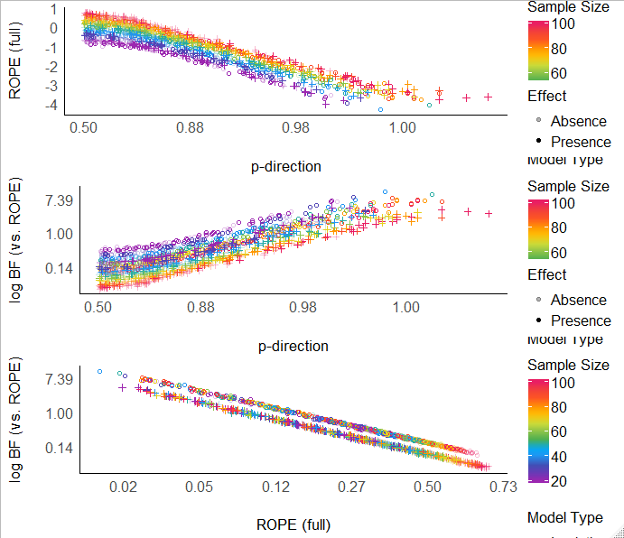
Now that I think of it, mathematically, the relationship between BF_rope and ROPE is:

BF_rope = odds(ROPE) / x
x = prior odds (a scalar as it depends on a priori information) (but in the BF perspective, this part is the most important part as it is what makes the BF represent a change from priors...).

from easystats.

Note in this figure that a BF of 1 is a ROPE of ~5%!
(Also BF of 1 is a pd of ~97.5%, which makes sense and previous work has shown that BF=1 is ~p-value=5%).

My current conclusions are: BF (mostly BF_rope, but also regular BF) and ROPE as measures are essentially interchangeable, the only difference being that BF accounts for prior knowledge - so use of which would depend on whether one thinks that information is important... The only question remaining in my opinions is: which criteria are better calibrated?

from easystats.

((Note that the relationship between BF and ROPE is only relevant in the context here of posterior based BF, not marginal likelihood BFs that are more flexible and would somewhat break and bend the interchangeability...))

from easystats.

based on all that, keeping the two extremes, bf rope and pd makes sense to me, the former drawing from the strengths of bfs and rope and the latter from its simplicity and familiar feel

I wonder what would be the sleekest way to textually report it

e. g. the effect has 98% of chance of being positive and can be considered as small (estim). There is moderate evidence in favour of its significance (BF = 11).

from easystats.

I would add that ROPE is better suited for "users" who have weak prior knowledge (reflected in the prior scale).

"A small effect was found (estimate + CI), with a pd% of chance of being positive, and was more favorable than the null effect (BF = BF)."

more favorable / more strongly supported by the data?

from easystats.

I would add that ROPE is better suited for "users" who have weak prior knowledge

Mmh right... but are rstanarm's prior considered as weak? For instance I, which use rstanarm's priors, should I use ROPE or BF ROPE?

and was more favorable than the null effect

Since we are testing against ROPE (in the case of BF ROPE), its more probable than not significance (significance as in outside the ROPE) isn't it?

from easystats.

Mmh right... but are rstanarm's prior considered as weak? For instance I, which use rstanarm's priors, should I use ROPE or BF ROPE?

I meant more on a theoretical level:

• If one would use basically any priors (i.e., if one uses rstanarm's defaults just because they are defaults) I would say use ROPE.
• If one put thought into their priors (type / scale / location) such that one thinks they are appropriate for their analysis, I would say use BF ROPE.

(This is also true for users of BayesFactor, where it is possible to set the prior width - but most just blindly use the defaults).

(This is my current conclusion from this simulation paper and overall working with you guys 😊 and why I tell my students and colleagues)

Too harsh?

How about:
"A [small/medium/large] effect was found (estimate + CI), with a pd% of chance of being [positive/negative], and was [more/less] favorable than a negligible effect (BF = BF)."

from easystats.

I understand your dual-index rule depending on the subjective importance of the prior, but I am afraid people will, in the end, stick to one because of habits, and probably BF ROPE because "OF COURSE I PUT SOME THOUGHT IN MY PRIORS" 😅

from easystats.

but BFs are sensitive to prior specification!

Gettin ready for study 2 & 3 about robustness to sampling parameters and priors specification 😬

from easystats.

from easystats.

https://twitter.com/StatModeling/status/1158362089515376645?s=20

Gelman's hole n°3: "Bayes factors don’t work" 😬

from easystats.

from easystats.

So I rebuild figure 1. All indices are transformed to log-odds (as done here and here), with the y-axis break labels on the "raw" scale. It looks like this:

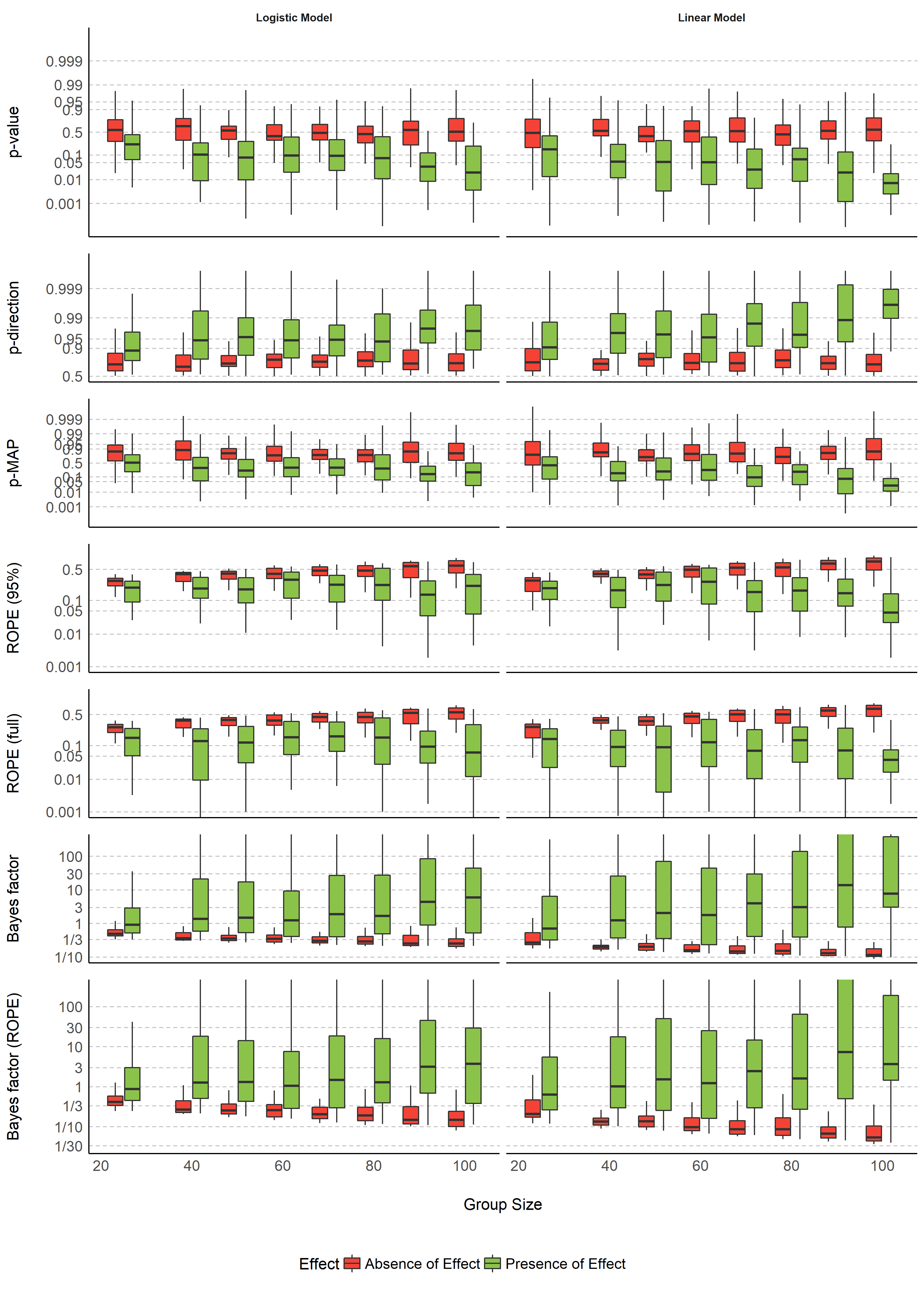
What do you guys think? Is this an avenue worth perusing (for the other plots as well)?

(I had to break the plot down into subplots and then put it back together with cowplot)

from easystats.

Nice, but in this case, shouldn't the y axis be unified for all of the indices? I don't know if it's very intuitive for the other indices to distort the scale, especially since the effect looked quite of sample size looked quite linear.

However, I agree that BFs expressed this way are better, and that the dashed lines corresponding to selected ticks make it more readable too. It's just the distortion of the axes that are potentially unnecessary?

from easystats.