Comments (12)
 cjekel
commented on May 22, 2024
1
cjekel
commented on May 22, 2024
1
For degree = 1, the beta vector is seen in Equation 4 https://github.com/cjekel/piecewise_linear_fit_py/blob/master/paper/pwlf_Jekel_Venter_v2.pdf
Essentially the order goes from left to right. The first value is the y intecept. The seocond value the slope, the third value is the change of slope of the next line, the fourth value is the change of slope between the third and second line...
I can give more detailed answer tomorrow.
from piecewise_linear_fit_py.
cjekel
commented on May 22, 2024
1
@cjekel thank you for your attention, could you provide more information about how to interpret my_pwlf.beta for n segments? I am really confused..
As in the example that i gave above, I got:
my_pwlf.beta: [-3.91201469e-07,  2.00000039e+00, -5.00000028e+00]
my_pwlf.fit_breaks: [0.        , 3.99999968, 9.        ]
my_pwlf.intercepts: [-3.91201469e-07,  1.99999991e+01]
my_pwlf.slopes: [ 2.00000039, -2.99999989]
For this my_pwlf.beta, how do I get the coefficients [2, 0] for the first segment and [-3, 20] for the second segment?
So in this case, the first line involves the first two parameters, where .beta[0] is the y-intercept, and .beta[1] is the slope. Then the second line is defined by .beta[2], where the slope of the second line is .beta[1] + .beta[2]. This pattern continues for additional line segments.
You could then use point-slope form to obtain the equations of each line.
Now for higher degrees which is a bit more complicated. I essentially assemble all of the degree=1 terms first, then all of the degree=2 second. The code to do this is in the assemble_regression_matrix method, and looks like this:
# Assemble the regression matrix
A_list = [np.ones_like(x)]
if self.degree >= 1:
A_list.append(x - self.fit_breaks[0])
for i in range(self.n_segments - 1):
A_list.append(np.where(x > self.fit_breaks[i+1],
x - self.fit_breaks[i+1],
0.0))
if self.degree >= 2:
for k in range(2, self.degree + 1):
A_list.append((x - self.fit_breaks[0])**k)
for i in range(self.n_segments - 1):
A_list.append(np.where(x > self.fit_breaks[i+1],
(x - self.fit_breaks[i+1])**k,
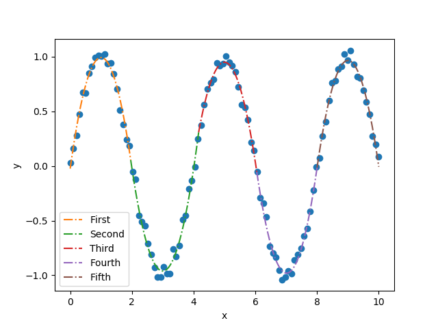
0.0))Let's take a look at this example which fits five line segments, each of degree=2. The mathematical equation of such a line is shown here. I've uploaded the jupyter notebook of this here.
import numpy as np
import pwlf
# generate sin wave data
x = np.linspace(0, 10, num=100)
y = np.sin(x * np.pi / 2)
# add noise to the data
y = np.random.normal(0, 0.05, 100) + y
my_pwlf_2 = pwlf.PiecewiseLinFit(x, y, degree=2)
res2 = my_pwlf_2.fitfast(5, pop=50)
The first line is defined by:
# first line
xhat = np.linspace(my_pwlf_2.fit_breaks[0], my_pwlf_2.fit_breaks[1], 100)
yhat = (my_pwlf_2.beta[0] +
        my_pwlf_2.beta[1]*(xhat-my_pwlf_2.fit_breaks[0]) +
        my_pwlf_2.beta[6]*(xhat-my_pwlf_2.fit_breaks[0])**2)
The second line is defined by:
# second segment
xhat2 = np.linspace(my_pwlf_2.fit_breaks[1], my_pwlf_2.fit_breaks[2], 100)
yhat2 = (my_pwlf_2.beta[0] +
         (my_pwlf_2.beta[1])*(xhat2-my_pwlf_2.fit_breaks[0]) +
         (my_pwlf_2.beta[2])*(xhat2-my_pwlf_2.fit_breaks[1]) +
         (my_pwlf_2.beta[6])*(xhat2-my_pwlf_2.fit_breaks[0])**2 +
         (my_pwlf_2.beta[7])*(xhat2-my_pwlf_2.fit_breaks[1])**2)
The third line is defined by:
# Third segment
xhat3 = np.linspace(my_pwlf_2.fit_breaks[2], my_pwlf_2.fit_breaks[3], 100)
yhat3 = (my_pwlf_2.beta[0] +
         (my_pwlf_2.beta[1])*(xhat3-my_pwlf_2.fit_breaks[0]) +
         (my_pwlf_2.beta[2])*(xhat3-my_pwlf_2.fit_breaks[1]) +
         (my_pwlf_2.beta[3])*(xhat3-my_pwlf_2.fit_breaks[2]) +
         (my_pwlf_2.beta[6])*(xhat3-my_pwlf_2.fit_breaks[0])**2 +
         (my_pwlf_2.beta[7])*(xhat3-my_pwlf_2.fit_breaks[1])**2 +
         (my_pwlf_2.beta[8])*(xhat3-my_pwlf_2.fit_breaks[2])**2)
The fourth line is defined by:
# Fourth segment
xhat4 = np.linspace(my_pwlf_2.fit_breaks[3], my_pwlf_2.fit_breaks[4], 100)
yhat4 = (my_pwlf_2.beta[0] +
         (my_pwlf_2.beta[1])*(xhat4-my_pwlf_2.fit_breaks[0]) +
         (my_pwlf_2.beta[2])*(xhat4-my_pwlf_2.fit_breaks[1]) +
         (my_pwlf_2.beta[3])*(xhat4-my_pwlf_2.fit_breaks[2]) +
         (my_pwlf_2.beta[4])*(xhat4-my_pwlf_2.fit_breaks[3]) +
         (my_pwlf_2.beta[6])*(xhat4-my_pwlf_2.fit_breaks[0])**2 +
         (my_pwlf_2.beta[7])*(xhat4-my_pwlf_2.fit_breaks[1])**2 +
         (my_pwlf_2.beta[8])*(xhat4-my_pwlf_2.fit_breaks[2])**2 +
         (my_pwlf_2.beta[9])*(xhat4-my_pwlf_2.fit_breaks[3])**2)
The fifth line is defined by:
# Fifth segment
xhat5 = np.linspace(my_pwlf_2.fit_breaks[4], my_pwlf_2.fit_breaks[5], 100)
yhat5 = (my_pwlf_2.beta[0] +
         (my_pwlf_2.beta[1])*(xhat5-my_pwlf_2.fit_breaks[0]) +
         (my_pwlf_2.beta[2])*(xhat5-my_pwlf_2.fit_breaks[1]) +
         (my_pwlf_2.beta[3])*(xhat5-my_pwlf_2.fit_breaks[2]) +
         (my_pwlf_2.beta[4])*(xhat5-my_pwlf_2.fit_breaks[3]) +
         (my_pwlf_2.beta[5])*(xhat5-my_pwlf_2.fit_breaks[4]) +
         (my_pwlf_2.beta[6])*(xhat5-my_pwlf_2.fit_breaks[0])**2 +
         (my_pwlf_2.beta[7])*(xhat5-my_pwlf_2.fit_breaks[1])**2 +
         (my_pwlf_2.beta[8])*(xhat5-my_pwlf_2.fit_breaks[2])**2 +
         (my_pwlf_2.beta[9])*(xhat5-my_pwlf_2.fit_breaks[3])**2 +
         (my_pwlf_2.beta[10])*(xhat5-my_pwlf_2.fit_breaks[4])**2)
And the final picture of the fit is
Hopefully this will help you understand how polynomial coefficients are handled in pwlf. When you look at the mathematical expression, pwlf.predict feels almost magical!
from piecewise_linear_fit_py.
 joaoantoniocardoso
commented on May 22, 2024
1
joaoantoniocardoso
commented on May 22, 2024
1
@cjekel Hi! wow, thank you so much, your explanation was very good and now I understood the standard of this beta coefficients.
In a similar math I was able to code a function to convert to the parameters in the way that I need in my application (y(x) = a + b*x + c*x^2 +...) so I have refactored this .ipynb gist to demonstrate it working.
But because it seems very complex to me to find a generalized pattern for a 'n' degree, it only works for degrees of 1 to 3, that fit very well in my application.
Again, thank you for such attention, you done an incredible job programming and explaining it, congrats!
from piecewise_linear_fit_py.
cjekel
commented on May 22, 2024
1
@joaoantoniocardoso I was looking at your ipynb and noticed that the very first data point has a discrepancy between predict and coeffs test? Is this an artifact in plotting, or a real discrepancy? If there is an issue, it appears it's only in the first segment.
I think perhaps the logic of test_coefs should be swapped to:
(x[i] >= breaks[segment]) and (x[i] < breaks[segment+1])Otherwise, your implementation shows that you have a full working understanding of this library!
I had an epiphany this morning about how to use sympy to construct these equations. (If you don't mind using sympy). It should work for degrees > 3 if you ever need them.
from sympy import Symbol
from sympy.utilities import lambdify
x = Symbol('x')

def get_symbolic_eqn(pwlf_, segment_number):
    if pwlf_.degree < 1:
        raise ValueError('Degree must be at least 1')
    if segment_number < 1 or segment_number > pwlf_.n_segments:
        raise ValueError('segment_number not possible')
    # assemble degree = 1 first
    for line in range(segment_number):
        if line == 0:
            my_eqn = pwlf_.beta[0] + (pwlf_.beta[1])*(x-pwlf_.fit_breaks[0])
        else:
            my_eqn += (pwlf_.beta[line+1])*(x-pwlf_.fit_breaks[line])
    # assemble all other degrees
    if pwlf_.degree > 1:
        for k in range(2, pwlf_.degree + 1):
            for line in range(segment_number):
                beta_index = pwlf_.n_segments*(k-1) + line + 1
                my_eqn += (pwlf_.beta[beta_index])*(x-pwlf_.fit_breaks[line])**k
    return my_eqn.simplify()
Note that you could improve the performance of this by saving the previous segment equation.
I added code to run this example at the end of this notebook
from piecewise_linear_fit_py.
cjekel
commented on May 22, 2024
1
I don't think (right now) I want to add sympy as a requirement to this library, but maybe I'll change my mind in the future.
At the very least, I should add this as an example, since people have asked about equations before.
You bring up a good point, let me reopen this until something is added to the library.
from piecewise_linear_fit_py.
cjekel
commented on May 22, 2024
1
Added example here e57d106
from piecewise_linear_fit_py.
cjekel
commented on May 22, 2024
The coefficients should be stored in my_pwlf.beta, you can also take a my_pwlf.slopes but it won't make sense with higher degree terms.
from piecewise_linear_fit_py.
joaoantoniocardoso
commented on May 22, 2024
@cjekel thank you for your attention, could you provide more information about how to interpret my_pwlf.beta for n segments? I am really confused..
As in the example that i gave above, I got:
my_pwlf.beta: [-3.91201469e-07,  2.00000039e+00, -5.00000028e+00]
my_pwlf.fit_breaks: [0.        , 3.99999968, 9.        ]
my_pwlf.intercepts: [-3.91201469e-07,  1.99999991e+01]
my_pwlf.slopes: [ 2.00000039, -2.99999989]
For this my_pwlf.beta, how do I get the coefficients [2, 0] for the first segment and [-3, 20] for the second segment?
from piecewise_linear_fit_py.
joaoantoniocardoso
commented on May 22, 2024
Maybe right now I got something - for a polynomial described as y(x) = a + b * x + c * x^2 + ..., the my_pwlf.beta is in this format:
beta = np.array([
    [???, # really didn't know what is this first element
    [b0, b1 - b0, b2 - b1 - b0, ...],
    [c0, c1 - c0, c2 - c1 - c0, ...],
    ...
]).flatten()
To illustrate how I would extract the coefficients from it:
print('Polynomial coefficient in a format of: y(x) = a + b*x + c*x^2 ...')

symbol = list('abcdefghijklmnopqrstuvwxyz')
betas = my_pwlf.beta[1:].reshape((my_pwlf.degree, my_pwlf.n_segments))
alphas = my_pwlf.intercepts

p = np.zeros((my_pwlf.degree + 1, my_pwlf.n_segments))

for segment in range(my_pwlf.n_segments):
    print(f'segment {segment}:')
    for coeff in range(my_pwlf.degree +1):
        if coeff is my_pwlf.degree:
            p[segment, coeff] = alphas[segment]
        else:
            p[segment, coeff] = betas[coeff-1,:segment+1].sum()
        print(f'\t {symbol[coeff]}{segment} = {p[segment, coeff]}')

print(p)
let me know if it is partially correct in some way
from piecewise_linear_fit_py.
joaoantoniocardoso
commented on May 22, 2024
Hi, I have refactored in a more organized way in this .ipynb gist.
So far I think my coefficients is not fully corrected because it fails at higher degree than 3 for some simple fake data. For some more complex (but smooth - continous) real data it is only working for degree = 1. Although the pwlf.predict() method is always working for these data for various degrees and segments.
I am kind new to all this regression stuff so I don't fully understand your paper yet, I would appreciate with some help to extract the correct coefficients in the classical format for polynomials.
Thanks again for your attention
from piecewise_linear_fit_py.
cjekel
commented on May 22, 2024
@joaoantoniocardoso Please let me know if this helps! I really need to update the paper. I've made some significant changes to the library since the 0.4.1 release that aren't covered in the paper.
from piecewise_linear_fit_py.
joaoantoniocardoso
commented on May 22, 2024
Man your solution is just amazing, I though going into this direction but I have a very limited time window for using this in a project so I didn't tried.. Don't you think that maybe it would be interest to add it to your library as a feature to be compatible with numpy.poly1d?
And yeah, you was right about test_coefs, thank you again!
from piecewise_linear_fit_py.
Related Issues (20)
- .fit() fails with 1 segment HOT 5
- How to force the fit process to have a fixed Intercept? HOT 1
- Can I get y_values if I have only x and slopes values? HOT 1
- Limit the slope of each segment of the curve HOT 1
- Re-constructing Piecewise PWLF HOT 2
- Set Slope of Segment to 0 HOT 2
- How to fit multiple functions simultaneously HOT 3
- Hi, i want to make sure that there are no fitted lines between points that are too far apart i.e. set a min value( fragment optimization) how to achieve this? HOT 1
- Why last beta is always positive? HOT 3
- How to prevent poor fitting HOT 4
- Forcing the segments to be integers and not float
- p values does not seem accurate HOT 3
- Error for coefficients of linear equations HOT 7
- pwlf with unknown line segments HOT 9
- assure the slopes to be lower and lower HOT 1
- divide by zero error in calc slopes if two break points are the same, or if a breakpoint is on the boundary HOT 2
- Issue using .fit() HOT 5
- How to plot segments with fit_breaks information HOT 4
- support random seed on init
- How to calculate prediction intervals? HOT 1
Recommend Projects
-
 React
React
A declarative, efficient, and flexible JavaScript library for building user interfaces.
-
Vue.js
🖖 Vue.js is a progressive, incrementally-adoptable JavaScript framework for building UI on the web.
-
 Typescript
TypeScript is a superset of JavaScript that compiles to clean JavaScript output.
-
TensorFlow
An Open Source Machine Learning Framework for Everyone
-
Django
The Web framework for perfectionists with deadlines.
-
 Laravel
A PHP framework for web artisans
-
D3
Bring data to life with SVG, Canvas and HTML. 📊📈🎉
-
Recommend Topics
-
javascript
JavaScript (JS) is a lightweight interpreted programming language with first-class functions.
-
web
Some thing interesting about web. New door for the world.
-
server
A server is a program made to process requests and deliver data to clients.
-
Machine learning
Machine learning is a way of modeling and interpreting data that allows a piece of software to respond intelligently.
-
Visualization
Some thing interesting about visualization, use data art
-
Game
Some thing interesting about game, make everyone happy.
Recommend Org
-
Facebook
We are working to build community through open source technology. NB: members must have two-factor auth.
-
Microsoft
Open source projects and samples from Microsoft.
-
Google
Google ❤️ Open Source for everyone.
-
Alibaba
Alibaba Open Source for everyone
-
D3
Data-Driven Documents codes.
-
Tencent
China tencent open source team.
from piecewise_linear_fit_py.