Introduction
General Usage
- Examples
Particle-In-Cell Method
- Functions
- Examples
Active Subspace Sensitivity Methods
- Functions
- Examples

Introduction

This repository is meant to allow for active subspace sensitivity analysis of plasma dynamics using a particle-in-cell (PIC) method.

General Usage

The PIC subdirectory contains two main functions - one is designed to create movies and images of phase-space dynamics, and the other is for creating the functions used in the sensitivity analysis. The folders Initilization and QOI_calc contain functions for initializing the particle distributions and calculating the quantities of interest, respectively.

The sensitivity subdirectory contains functions for gradient-based and linear-fit sensitivity metrics. Associated functions designed to create plots based on the data are also included.

Examples

Usage examples for two Landau Damping and one Two-Stream Instability (split into two parts - one with a tight beam and one without) are included.

Particle-In-Cell Method

Using typical parameter values of ..., each evaluation of the PIC algorithm takes approximately five minutes. Time complexity of the algorithm is roughly quadratic in number of particles, linear in number of spatial gridpoints, and linear in both temporal gridpoints and maximal value. It's recommended that when using the movie_run.m more accurate particles and spatial gridpoints are used to ensure proper resolution. Maximal time is also taken in all examples to be close to the minimum possible, and longer time tends to show more clearly the dynamics.

Functions

movie_run( DT, NT, NG, N, distribution, params, saveFrameNum, movieFrameNum)

Parameter	Meaning
`DT`	Temporal step size
`NT`	Number of temporal steps
`NG`	Number of spatial gridpoints
`N`	Number of computational particles
`distribution`	Name of the distribution - for use in determining which functions to use in the `Initilization` and `QOI_calc` folders
`params`	Parameters for the initilization of the distribution - the spatial length is assumed to come first
`saveFrameNum`	Saves a .png file of the phase-space dynamics at every `saveFrameNum` temporal step (must be a multiple of `movieFrameNum`)
`movieFrameNum`	Adds a frame to the .mp4 movie of phase-space dynamics at every `movieFrameNum` temporal step

Used to generate still images and movies of phase-space behavior. Additionally generates plots of the behavior of energy using the second Fourier mode, L2 norm of the electric field, the kinetic energy, the potential energy, and the total energy. Uses a histcn function developed by Bruno Luong. Since maximum boundaries for the velocity are not known, an estimate is used - true values for the maximum and minimum are printed by the function to allow for hard-coded boundaries if this is inaccurate.

PIC = PIC_setup(DT, NT, NG, N, distribution)

Parameter	Meaning
`DT`	Temporal step size
`NT`	Number of temporal steps
`NG`	Number of spatial gridpoints
`N`	Number of computational particles
`distribution`	Name of the distribution - for use in determining which functions to use in the `Initilization` and `QOI_calc` folders

Sets up various constant values for use in a PIC function. Returns a PIC evaluator that accepts a parameter array for use in the initilization function in the Initilization folder. The length parameter is assumed to come first in this array. The PIC evaluator returns a metric from the function related to the distribution in the QOI_calc folder.

Examples

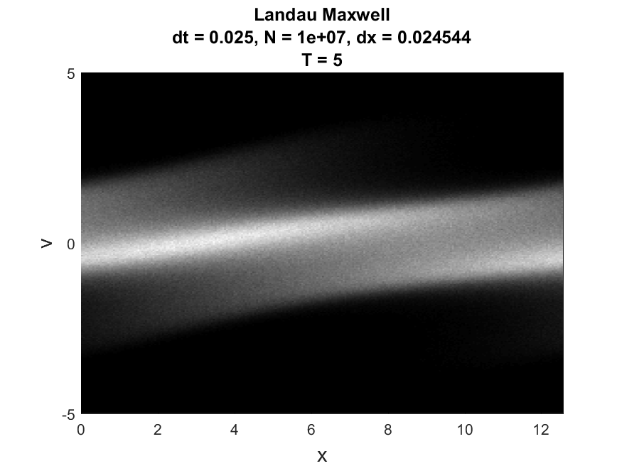
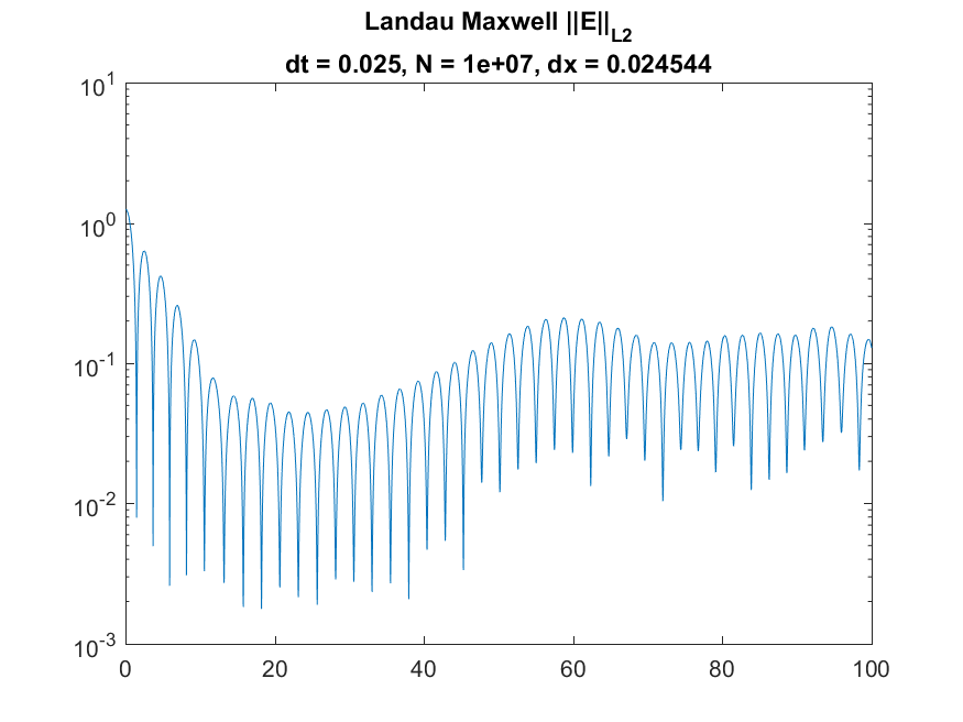
Examples are available for the Two-Stream Instability case and for the Landau damping case using either a Maxwellian or Lorentzian distribution. Examples of images for the Maxwellian case, contained in /Landau_Maxwell/imagesA05, are

Maxwellian L2-norm of the electric field

Active Subspace Sensitivity Methods

Functions

[evalues, U, output, outputplus, Xs, graddamp, sdev, Atrials] = FD_Gradient(max_vals, min_vals, h, Nsamples, func, varargin)

This function uses finite-differencing of the function of interest to calculate the computational gradient matrix.

Required Parameters	Meaning
`max_vals`	Upper bound of the range of tested parameter values
`min_vals`	Lower bound of the range of tested parameter values
`h`	Finite differencing step size for the approximation of the gradient matrix
`Nsamples`	Number of parameter samples to draw from to generate data points
`func`	The function the sensitivity metric is considered on - accepts a parameter vector of the from of `max_vals` and `min_vals` and outputs a numeric value

Optional Parameters	Use
`test_params`	A boolean vector - false represents a parameter that is constant and true represents a parameter to be tested. Defaults to a vector of ones.
`Averaging`	A boolean value - false means each data point is absolute, true means each data point is approximated by a mean value of repeated function runs. Defaults to false.
`Asamples`	Number of samples to use with averaging - a mean is generated by running the function for each parameter set this many times. Defaults to 10 if averaging is used.
`Atolerance`	Maximum standard deviation allowed for each data point mean estimation. Can be used with `Asamples` and defaults to infinity.

Output	Meaning
`evalues`	A vector containing the eigenvalues of the computational gradient matrix in descending order.
`U`	A matrix of the associated eigenvectors - U(:, 1) contains the eigenvector corresponding to the largest eigenvalue.
`output`	A vector containing the quantity of interest at each data point
`outputplus`	A matrix containing the quantity of interest at each perturbation of the parameter values
`Xs`	A matrix containing the normalized weights used to compute each randomly selected parameter value
`graddamp`	The computational gradient matrix
`sdev`	A matrix containing the standard deviations of each estimated mean - for use with averaging
`Atrials`	A matrix containing the number of trials used to calculate each estimated mean - for use with averaging

plotter_FD_Gradient(Nparams, Nsamples, paramNames, QOI, evalues, U, output, Xs)

Parameter	Meaning
`Nparams`	Number of parameters tested in the gradient-based method
`Nsamples`	Number of samples used
`paramNames`	A string vector of the parameter names
`QOI`	A string containing the name of the quantity of interest
`evalues`	The eigenvalues of the computational gradient matrix
`U`	The matrix containing the associated eigenvectors
`output`	The vector containing the quantity of intest at each data point
`Xs`	The matrix containing the normalized weights used to compute each randomly selected parameter value

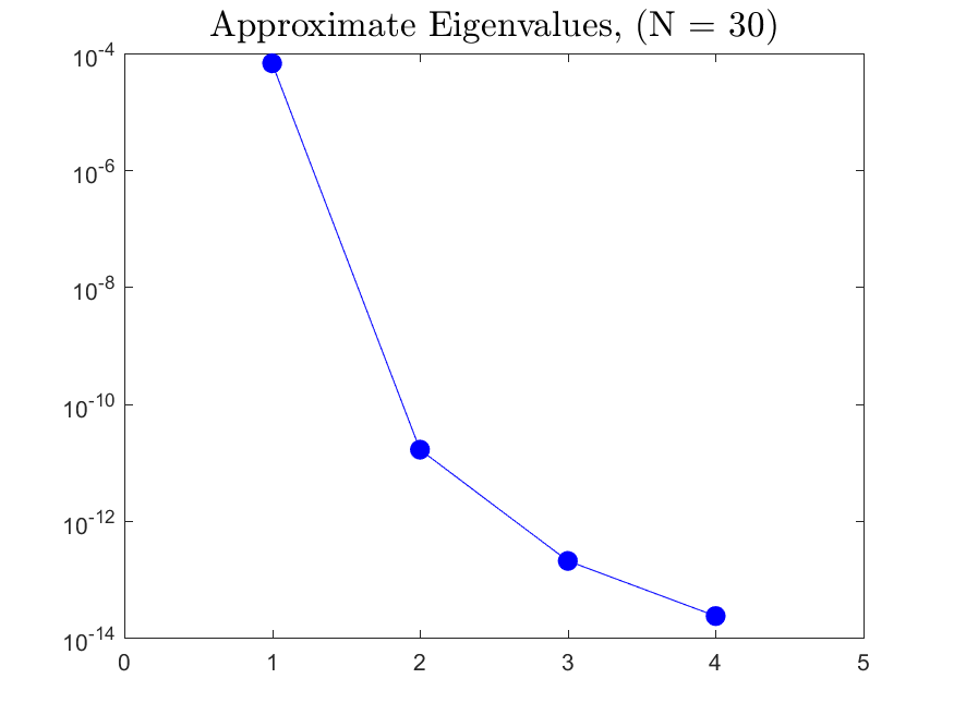
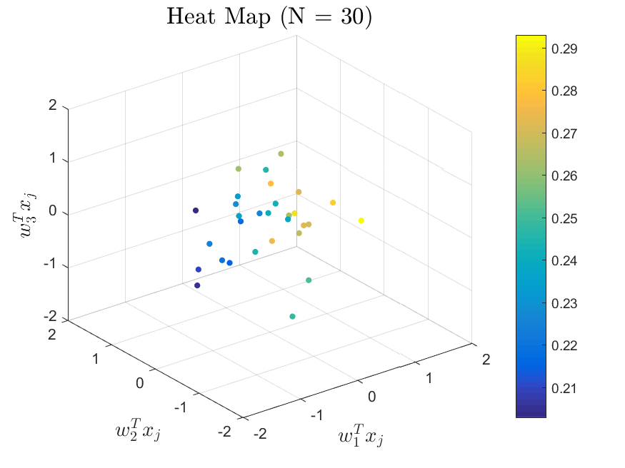
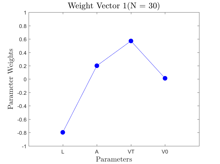
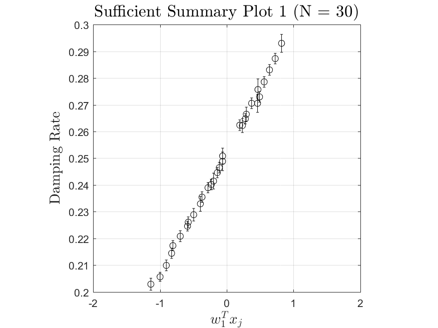
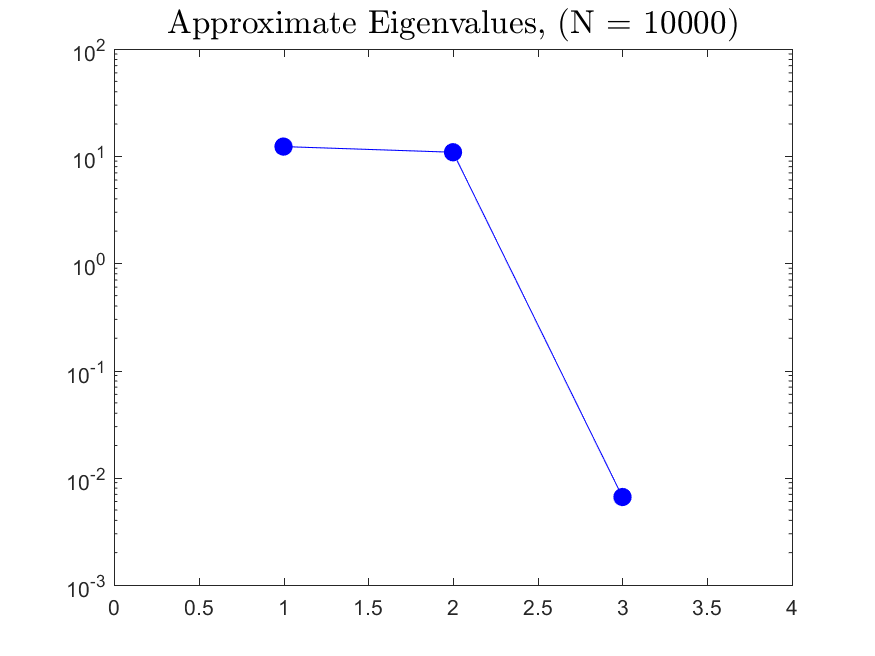
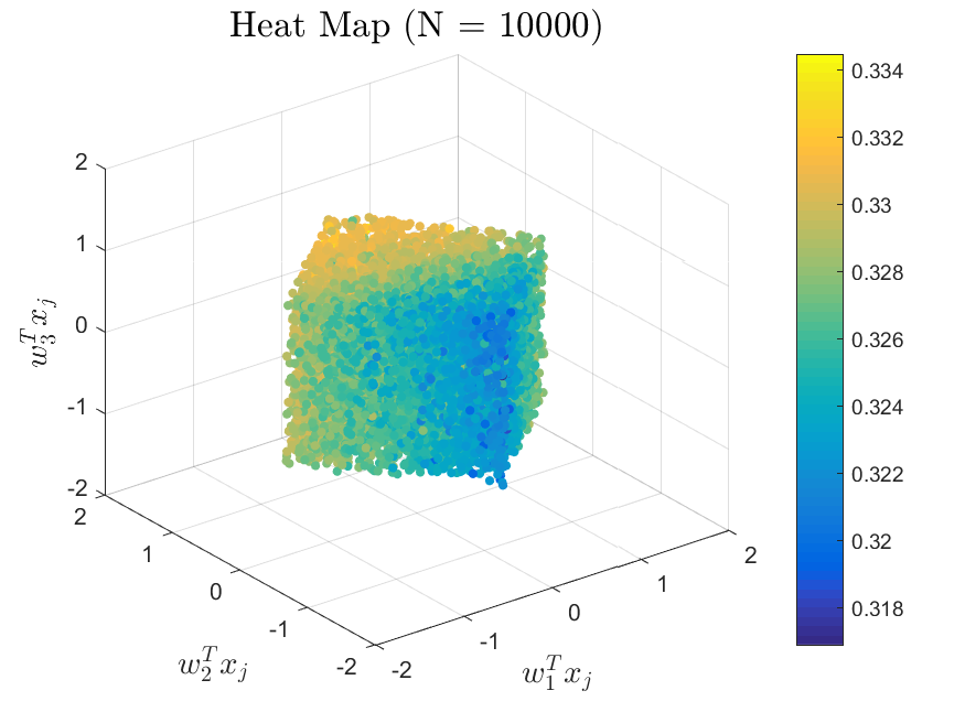
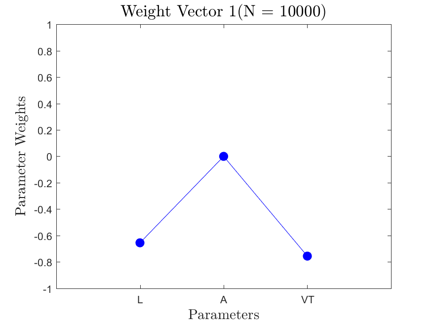
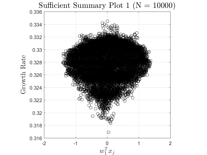
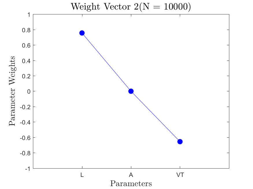
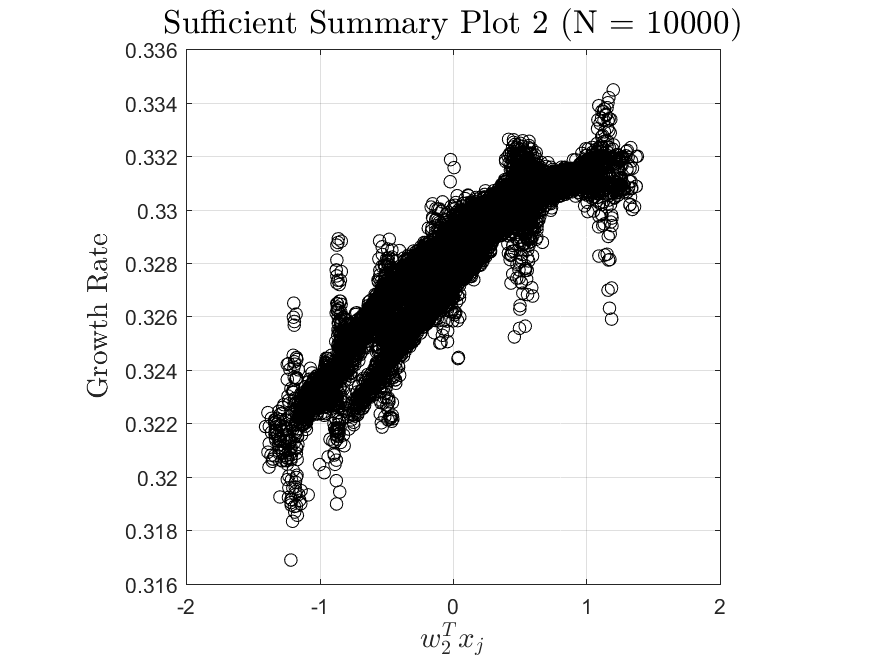
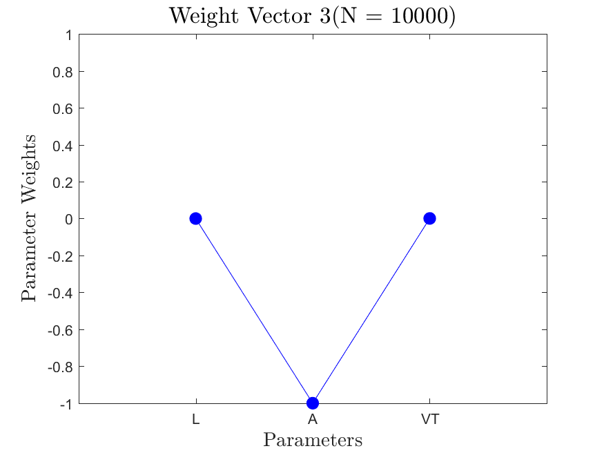
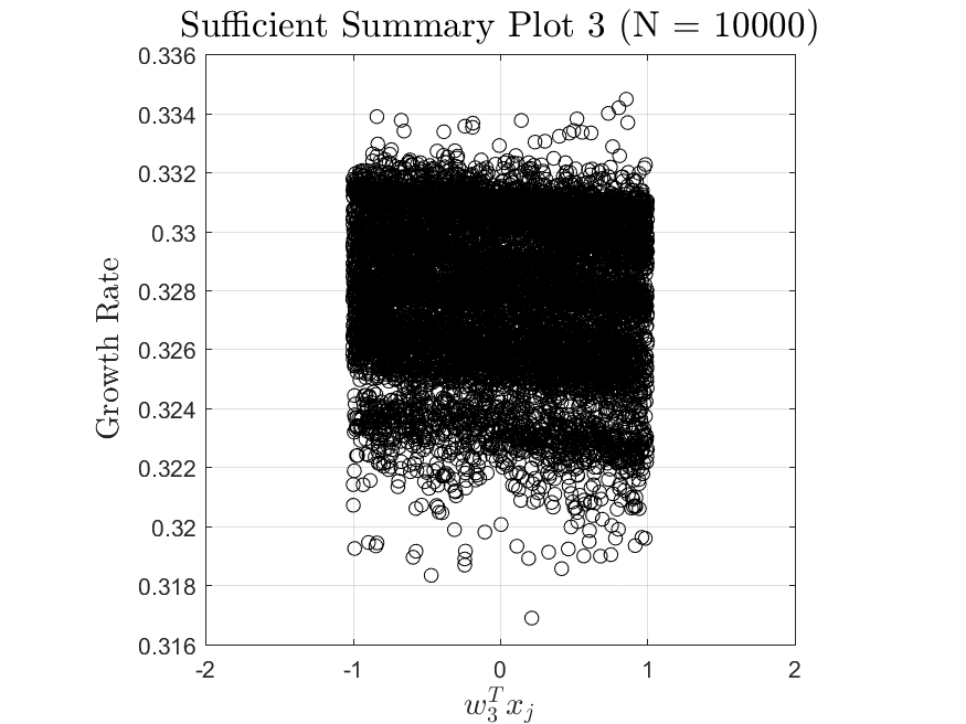
This function is meant to be used with the Active_Subspaces function. It generates, displays, and saves figures related to active subspace metrics. Specifically, it plots the eigenvectors on a logarithmic scale, plots the weight vectors and sufficient summary plots for each weighting, and if there are three or more parameters it generates a three-dimensional heat map of the first three eigenvectors.

[evalues, U, output, Xs, Xs2, graddamp, sdev, Atrials] = Local_Linear_Model(max_vals, min_vals, Nsamples, Nsamples2, p, func, varargin)

This function uses local linear regression models to calculate the computational gradient matrix.

Required Parameters	Meaning
`max_vals`	Upper bound of the range of tested parameter values
`min_vals`	Lower bound of the range of tested parameter values
`Nsamples`	Number of parameter samples to draw from to generate data points
`Nsamples2`	Number of parameter samples to draw from for locations for the local linear models
`p`	Number of parameter samples to draw from to generate data points, `Nsamples2` < `p` < `Nsamples`
`func`	The function the sensitivity metric is considered on - accepts a parameter vector of the from of `max_vals` and `min_vals` and outputs a numeric value

Optional Parameters	Use
`test_params`	A boolean vector - false represents a parameter that is constant and true represents a parameter to be tested. Defaults to a vector of ones.
`Averaging`	A boolean value - false means each data point is absolute, true means each data point is approximated by a mean value of repeated function runs. Defaults to false.
`Asamples`	Number of samples to use with averaging - a mean is generated by running the function for each parameter set this many times. Defaults to 10 if averaging is used.
`Atolerance`	Maximum standard deviation allowed for each data point mean estimation. Can be used with `Asamples` and defaults to infinity.

Output	Meaning
`evalues`	A vector containing the eigenvalues of the computational gradient matrix in descending order.
`U`	A matrix of the associated eigenvectors - U(:, 1) contains the eigenvector corresponding to the largest eigenvalue.
`output`	A vector containing the quantity of interest at each data point
`Xs`	A matrix containing the normalized weights used to compute each randomly selected parameter value
`Xs`	A matrix containing the locations in the parameter space of the local linear model locations
`graddamp`	The computational gradient matrix
`sdev`	A matrix containing the standard deviations of each estimated mean - for use with averaging
`Atrials`	A matrix containing the number of trials used to calculate each estimated mean - for use with averaging

plotter_Local_Linear_Model(Nparams, Nsamples, paramNames, QOI, evalues, U, output, Xs, varargin)

Parameter	Meaning
`Nparams`	Number of parameters tested in the gradient-based method
`Nsamples`	Number of samples used
`paramNames`	A string vector of the parameter names
`QOI`	A string containing the name of the quantity of interest
`evalues`	The eigenvalues of the computational gradient matrix
`U`	The matrix containing the associated eigenvectors
`output`	The vector containing the quantity of intest at each data point
`Xs`	The matrix containing the normalized weights used to compute each randomly selected parameter value

This function is meant to be used with the Local_Linear_Model function. It generates, displays, and saves figures related to active subspace metrics. Specifically, it plots the eigenvectors on a logarithmic scale, plots the weight vectors and sufficient summary plots for each weighting, and if there are three or more parameters it generates a three-dimensional heat map of the first three eigenvectors. Optionally, the sdev vector can be passed in to generate errorbars on the sufficient summary plots.

[w, output, Xs, sdev, Atrials] = Linear_Fit(max_vals, min_vals, Nsamples, func, varargin)

Required Parameters	Meaning
`max_vals`	Upper bound of the range of tested parameter values
`min_vals`	Lower bound of the range of tested parameter values
`Nsamples`	Number of parameter samples to draw from to generate data points
`func`	The function the sensitivity metric is considered on - accepts a parameter vector of the from of `max_vals` and `min_vals` and outputs a numeric value

Optional Parameters	Use
`test_params`	A boolean vector - false represents a parameter that is constant and true represents a parameter to be tested. Defaults to a vector of ones.
`Averaging`	A boolean value - false means each data point is absolute, true means each data point is approximated by a mean value of repeated function runs. Defaults to false.
`Asamples`	Number of samples to use with averaging - a mean is generated by running the function for each parameter set this many times. Defaults to 10 if averaging is used.
`Atolerance`	Maximum standard deviation allowed for each data point mean estimation. Can be used with `Asamples` and defaults to infinity.

Output	Meaning
`w`	The relative weight of each parameter
`output`	A vector containing the quantity of interest at each data point
`Xs`	A matrix containing the normalized weights used to compute each randomly selected parameter value
`sdev`	A vector containing the standard deviations of each estimated mean - for use with averaging
`Atrials`	A vector containing the number of trials used to calculate each estimated mean - for use with averaging

plotter_Linear_Fit(Nparams, Nsamples, paramNames, QOI, w, output, Xs, varargin)

Parameter	Meaning
`Nparams`	Number of parameters tested in the gradient-based method
`Nsamples`	Number of samples used
`paramNames`	A string vector of the parameter names
`QOI`	A string containing the name of the quantity of interest
`w`	The relative weight of each parameter
`output`	The vector containing the quantity of intest at each data point
`Xs`	The matrix containing the normalized weights used to compute each randomly selected parameter value

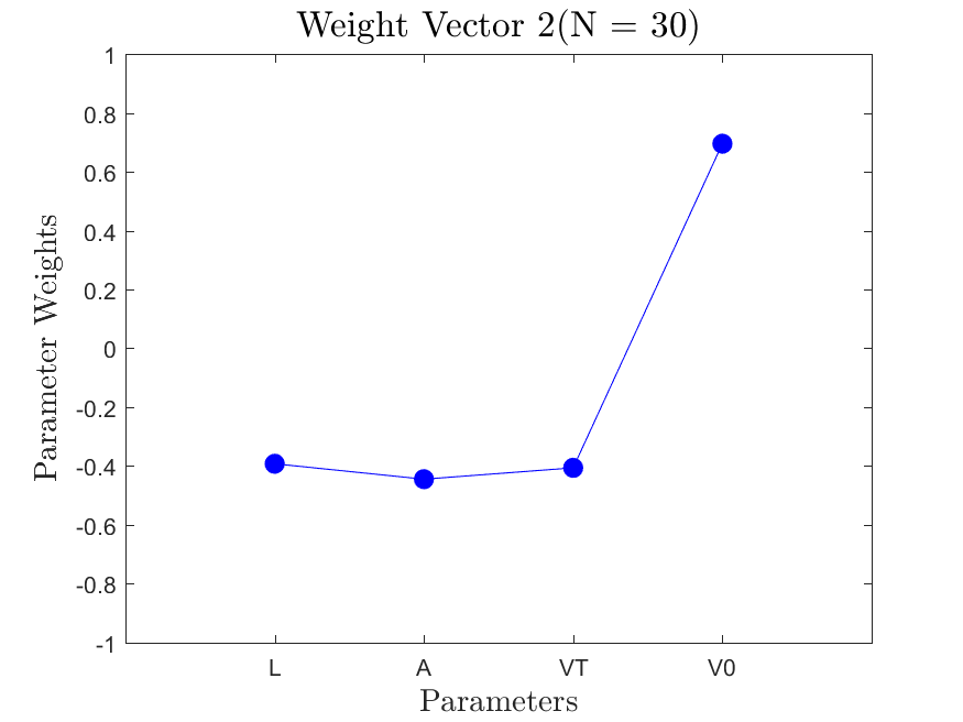
This function is meant to be used with the Linear_Fit function. It generates, displays, and saves a plot of the weight vector and associated sufficient summary plot. Optionally, the sdev vector can be passed in to generate errorbars on the sufficient summary plot.

Examples

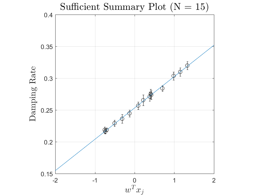
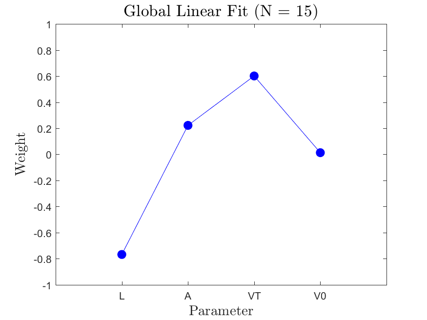
All the distributions have linear models with code in the <distribution>_LF.m files and results in the Results_LF subfolders of each distribution. Examples of linear fit results for the Maxwellian distribution are

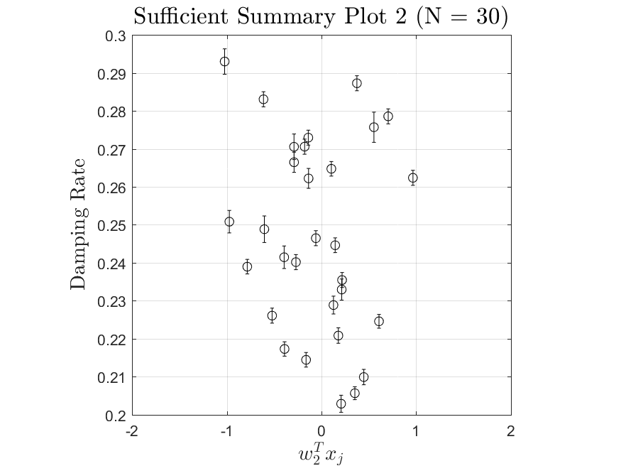
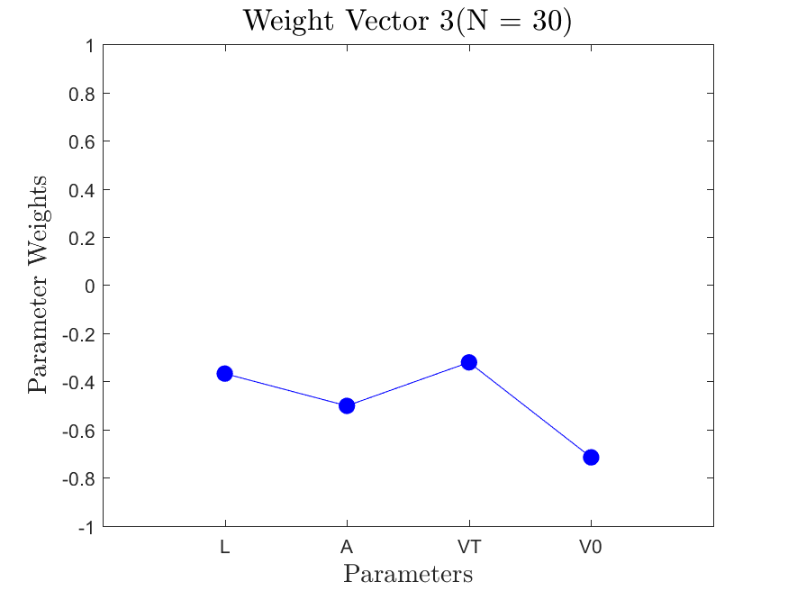
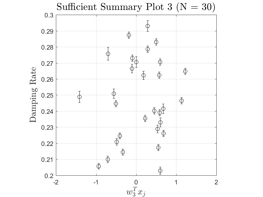
All the distributions also have local linear regression models with code in the <distribution>_LLRM.m files and results in the Results_LLRM subfolders of each distribution. Examples of regression model results for the Maxwellian distribution are

The Two-Stream with no variance has results for the gradient-based active subspace model. The Maxwellian Landau Damping case also has results, but they are not refined enough to be useable (the finite differencing step-size to approximate the gradient matrix cannot be taken small enough without making computations infeasible). Examples of the output of the Two-Stream case are